This edition applies to the version 3, release 0 of the IBM Software Development Kit for Multicore Acceleration (Product number 5724-S84) and to all subsequent releases and modifications until otherwise indicated in new editions.
This edition replaces SC33-8325-01.
The IBM Software Development Kit for Multicore Acceleration Version 3.0 (SDK 3.0) is a complete package of tools to enable you to program applications for the Cell Broadband Engine(TM) (Cell BE) processor. The SDK 3.0 is composed of development tool chains, software libraries and sample source files, a system simulator, and a Linux(R) kernel, all of which fully support the capabilities of the Cell BE.
This book describes how to use the SDK 3.0 to write applications. How to install SDK 3.0 is described in a separate manual, Software Development Kit for Multicore Acceleration Version 3.0 Installation Guide, and there is also a programming tutorial to help get you started.
Each section of this book covers a different topic:
This book includes information about the new functionality delivered with the SDK 3.0, and completely replaces the previous version of this book. This new information includes:
For information about differences between SDK 3.0 and previous versions, see Appendix A. Changes to SDK for this release.
Cell BE applications can be developed on the following platforms:
The supported languages are:
This publication contains documentation that may be applied to certain environments on an "as-is" basis. Those environments are not supported by IBM, but wherever possible, workarounds to problems are provided in the respective forums.
The SDK 3.0 is available through Passport Advantage(R) with full support at:
http://www.ibm.com/software/passportadvantage
You can locate documentation and other resources on the World Wide Web. Refer to the following Web sites:
http://www.ibm.com/bladecenter/For service information, select Support.
http://www.ibm.com/developerworks/power/cell/To access the Cell BE forum on developerWorks, select Community.
http://www.bsc.es/projects/deepcomputing/linuxoncell
http://www.gnu.org/software/gdb/gdb.html
This version (SDK 3.0) of the SDK supersedes all previous versions of the SDK.
For a list of documentation referenced in this Programmer's Guide, see Appendix B. Related documentation.
This section describes the contents of the SDK 3.0, where it is installed on the system, and how the various components work together. It covers the following topics:
The GNU tool chain contains the GCC C-language compiler (GCC compiler) for the PPU and the SPU. For the PPU it is a replacement for the native GCC compiler on PowerPC (PPC) platforms and it is a cross-compiler on X86. The GCC compiler for the PPU is the default and the Makefiles are configured to use it when building the libraries and samples.
The GCC compiler also contains a separate SPE cross-compiler that supports the standards defined in the following documents:
The associated assembler and linker additionally support the SPU Assembly Language Specification V1.6. The assembler and linker are common to both the GCC compiler and the IBM XL C/C++ compiler.
GDB support is provided for both PPU and SPU debugging, and the debugger client can be in the same process or a remote process. GDB also supports combined (PPU and SPU) debugging.
On a non-PPC system, the install directory for the GNU tool chain is /opt/cell/toolchain. There is a single bin subdirectory, which contains both PPU and SPU tools.
On a PPC64 or BladeCenter QS21, both tool chains are installed into /usr. See System root directories for further information.
IBM XL C/C++ for Multicore Acceleration for Linux is an advanced, high-performance cross-compiler that is tuned for the CBEA. The XL C/C++ compiler, which is hosted on an x86, IBM PowerPC technology-based system, or a BladeCenter QS21, generates code for the PPU or SPU. The compiler requires the GCC toolchain for the CBEA, which provides tools for cross-assembling and cross-linking applications for both the PPE and SPE.
IBM XL C/C++ supports the revised 2003 International C++ Standard ISO/IEC 14882:2003(E), Programming Languages -- C++ and the ISO/IEC 9899:1999, Programming Languages -- C standard, also known as C99. The compiler also supports:
The XL C/C++ compiler available for the SDK 3.0 supports the languages extensions as specified in the IBM XL C/C++ Advanced Edition for Multicore Acceleration for Linux V9.0 Language Reference.
The XL compiler also contains a separate SPE cross-compiler that supports the standards defined in the following documents:
For information about the XL C/C++ compiler invocation commands and a complete list of options, refer to the IBM XL C/C++ Advanced Edition for Multicore Acceleration for Linux V9.0 Compiler Reference.
Program optimization is described in IBM XL C/C++ Advanced Edition for Multicore Acceleration for Linux V9.0 Programming Guide.
The XL C/C++ for Multicore Acceleration for Linux compiler is installed into the/opt/ibmcmp/xlc/cbe/<compiler version number> directory. Documentation is located on the following Web site:
http://publib.boulder.ibm.com/infocenter/cellcomp/v9v111/index.jsp
The IBM Full-System Simulator (referred to as the simulator in this document) is a software application that emulates the behavior of a full system that contains a Cell BE processor. You can start a Linux operating system on the simulator and run applications on the simulated operating system. The simulator also supports the loading and running of statically-linked executable programs and standalone tests without an underlying operating system.
The simulator infrastructure is designed for modeling processor and system-level architecture at levels of abstraction, which vary from functional to performance simulation models with a number of hybrid fidelity points in between:
This simulation model is useful for software development and debugging when a precise measure of execution time is not significant. Functional simulation proceeds much more rapidly than performance simulation, and so is also useful for fast-forwarding to a specific point of interest.
Operation latencies are modeled dynamically to account for both processing time and resource constraints. Performance simulation models have been correlated against hardware or other references to acceptable levels of tolerance.
The simulator for the Cell BE processor provides a cycle-accurate SPU core model that can be used for performance analysis of computationally-intense applications. The simulator for SDK 3.0 provides additional support for performance simulation. This is described in the IBM Full-System Simulator Users Guide.
The simulator can also be configured to fast-forward the simulation, using a functional model, to a specific point of interest in the application and to switch to a timing-accurate mode to conduct performance studies. This means that various types of operational details can be gathered to help you understand real-world hardware and software systems.
See the /opt/ibm/systemsim-cell/doc subdirectory for complete documentation including the simulator user's guide. The prerelease name of the simulator is "Mambo" and this name may appear in some of the documentation.
The simulator for the Cell BE processor is also available as an independent technology at
http://www.alphaworks.ibm.com/tech/cellsystemsim
The system root image for the simulator is a file that contains a disk image of Fedora 7 files, libraries, and binaries that can be used within the system simulator. This disk image file is preloaded with a full range of Fedora 7 utilities and also includes all of the Cell BE Linux support libraries described in Performance support libraries and utilities.
This RPM file is the largest of the RPM files and when it is installed, it takes up to 1.6 GB on the host server's hard disk. See also System root directories.
The system root image for the simulator must be located either in the current directory when you start the simulator or the default /opt/ibm/systemsim-cell/images/cell directory. The cellsdk script automatically puts the system root image into the default directory.
You can mount the system root image to see what it contains. Assuming a mount point of /mnt/cell-sdk-sysroot, which is the mount point used by the cellsdk_sync_simulator script, the command to mount the system root image is:
mount -o loop /opt/ibm/systemsim-cell/images/cell/sysroot_disk /mnt/cell-sdk-sysroot/
The command to unmount the image is:
umount /mnt/cell-sdk-sysroot/
Do not attempt to mount the image on the host system while the simulator is running. You should always unmount the system root image before you start the simulator. You should not mount the system root image to the same point as the root on the host server because the system can become corrupted and fail to boot.
You can change files on the system root image disk in the following ways:
For the BladeCenter QS21, the kernel is installed into the /boot directory, yaboot.conf is modified and a reboot is required to activate this kernel. The cellsdk install task is documented in the SDK 3.0 Installation Guide.
The following libraries are described in this section:
The SPE Runtime Management Library (libspe) constitutes the standardized low-level application programming interface (API) for application access to the Cell BE SPEs. This library provides an API to manage SPEs that is neutral with respect to the underlying operating system and its methods. Implementations of this library can provide additional functionality that allows for access to operating system or implementation-dependent aspects of SPE runtime management. These capabilities are not subject to standardization and their use may lead to non-portable code and dependencies on certain implemented versions of the library.
The elfspe is a PPE program that allows an SPE program to run directly from a Linux command prompt without needing a PPE application to create an SPE thread and wait for it to complete.
For the BladeCenter QS21, the SDK installs the libspe headers, libraries, and binaries into the /usr directory and the standalone SPE executive, elfspe, is registered with the kernel during boot by commands added to /etc/rc.d/init.d using the binfmt_misc facility.
For the simulator, the libspe and elfspe binaries and libraries are preinstalled in the same directories in the system root image and no further action is required at install time.
SPE Runtime Management Library version 2.2 is an upgrade to version 2.1. For more information, see the SPE Runtime Management Library Reference.
The traditional math functions are scalar instructions, and do not take advantage of the powerful Single Instruction, Multiple Data (SIMD) vector instructions available in both the PPU and SPU in the Cell BE Architecture. SIMD instructions perform computations on short vectors of data in parallel, instead of on individual scalar data elements. They often provide significant increases in program speed because more computation can be done with fewer instructions.
The SIMD math library provides short vector versions of the math functions. The MASS library provides long vector versions. These vector versions conform as closely as possible to the specifications set out by the scalar standards.
The SIMD math library is provided by the SDK as both a linkable library archive and as a set of inline function headers. The names of the SIMD math functions are formed from the names of the scalar counterparts by appending a vector type suffix to the standard scalar function name. For example, the SIMD version of the absolute value function abs(), which acts on a vector of long integers, is called absi4(). Inline versions of functions are prefixed with the character "_" (underscore), so the inline version of absi4() is called _absi4().
For more information about the SIMD math library, refer to SIMD Math Library Specification for Cell Broadband Engine Architecture Version 1.1.
The Mathematical Acceleration Subsystem (MASS) consists of libraries of mathematical intrinsic functions, which are tuned specifically for optimum performance on the Cell BE processor. Currently the 32-bit, 64-bit PPU, and SPU libraries are supported.
These libraries:
You can find information about using these libraries on the MASS Web site:
http://www.ibm.com/software/awdtools/mass
The ALF provides a programming environment for data and task parallel applications and libraries. The ALF API provides library developers with a set of interfaces to simplify library development on heterogenous multi-core systems. Library developers can use the provided framework to offload computationally intensive work to the accelerators. More complex applications can be developed by combining the several function offload libraries. Application programmers can also choose to implement their applications directly to the ALF interface.
ALF supports the multiple-program-multiple-data (MPMD) programming module where multiple programs can be scheduled to run on multiple accelerator elements at the same time.
The ALF functionality includes:
With the provided platform-independent API, you can also create descriptions for multiple compute tasks and define their ordering information execution orders by defining task dependency. Task parallelism is accomplished by having tasks without direct or indirect dependencies between them. The ALF runtime provides an optimal parallel scheduling scheme for the tasks based on given dependencies.
From the application or library programmer's point of view, ALF consists of the following two runtime components:
The host runtime library provides the host APIs to the application. The accelerator runtime library provides the APIs to the application's accelerator code, usually the computational kernel and helper routines. This division of labor enables programmers to specialize in different parts of a given parallel workload.
The ALF design enables a separation of work. There are three distinct types of task within a given application:
The runtime framework handles the underlying task management, data movement, and error handling, which means that the focus is on the kernel and the data partitioning, not the direct memory access (DMA) list creation or the lock management on the work queue.
The ALF APIs are platform-independent and their design is based on the fact that many applications targeted for Cell BE or multi-core computing follow the general usage pattern of dividing a set of data into self-contained blocks, creating a list of data blocks to be computed on the SPE, and then managing the distribution of that data to the various SPE processes. This type of control and compute process usage scenario, along with the corresponding work queue definition, are the fundamental abstractions in ALF.
The DaCS library provides a set of services for handling process-to-process communication in a heterogeneous multi-core system. In addition to the basic message passing service these include:
The DaCS services are implemented as a set of APIs providing an architecturally neutral layer for application developers They structure the processing elements, referred to as DaCS Elements (DE), into a hierarchical topology. This includes general purpose elements, referred to as Host Elements (HE), and special processing elements, referred to as Accelerator Elements (AE). Host elements usually run a full operating system and submit work to the specialized processes which run in the Accelerator Elements.
This section provides an overview of the following prototype libraries, which are shipped with SDK 3.0:
This prototype library handles a wide range of FFTs, and consists of the following:
The implementation manages sizes up to 10000 and handles multiples of 2, 3, and 5 as well as powers of those factors, plus one arbitrary factor as well. User code running on the PPU makes use of the CBE FFT library by calling one of either 1D or 2D streaming functions.
Both parts of the library run using a common interface that contains an initialization and termination step, and an execution step which can process "one-at-a-time" requests (streaming) or entire arrays of requests (batch).
Enter the following to view additional documentation for the prototype FFT library:
man /opt/cell/sdk/prototype/usr/include/libfft.3
The Monte Carlo libraries are a Cell BE implementation of Random Number Generator (RNG) algorithms and transforms. The objective of this library is to provide functions needed to perform Monte Carlo simulations.
The following RNG algorithms are implemented:
The following transforms are provided:
The example libraries package provides a set of optimized library routines that greatly reduce the development cost and enhance the performance of Cell BE programs.
To demonstrate the versatility of the Cell BE architecture, a variety of application-oriented libraries are included, such as:
Additional examples and demos show how you can exploit the on-chip computational capacity.
Both the binary and the source code are shipped in separate RPMs. The RPM names are:
For each of these, there is one RPM that has the binaries - already built versions, that are installed into /opt/cell/sdk/usr, and for each of these, there is one RPM that has the source in a tar file. For example, cell-demos-source-3.0-1.rpm has demos_source.tar and this tar file contains all of the source code.
The default installation process installs the binaries and installs the source tar files. You need to decide into which directory you want to untar those files, either into /opt/cell/sdk/src, or into a 'sandbox' directory.
The libraries and examples RPMs have been partitioned into the following subdirectories.
The following support libraries and utilities are provided by the SDK to help you with development and performance testing your Cell BE applications.
The SPU static timing tool, spu_timing, annotates an SPU assembly file with scheduling, timing, and instruction issue estimates assuming a straight, linear execution of the program. The tool generates a textual output of the execution pipeline of the SPE instruction stream from this input assembly file. Run spu_timing --help to see its usage syntax.
The SPU timing tool is located in the /opt/cell/sdk/usr/bin directory.
OProfile is a tool for profiling user and kernel level code. It uses the hardware performance counters to sample the program counter every N events. You specify the value of N as part of the event specification. The system enforces a minimum value on N to ensure the system does not get completely swamped trying to capture a profile.
Make sure you select a large enough value of N to ensure the overhead of collecting the profile is not excessively high.
The opreport tool produces the output report. Reports can be generated based on the file names that correspond to the samples, symbol names or annotated source code listings.
How to use OProfile and the postprocessing tool is described in the user manual available at:
http://oprofile.sourceforge.net/doc/
The current SDK 3.0 version of OProfile for Cell BE supports profiling on the POWER(TM) processor events and SPU cycle profiling. These events include cycles as well as the various processor, cache and memory events. It is possible to profile on up to four events simultaneously on the Cell BE system. There are restrictions on which of the PPU events can be measured simultaneously. (The tool now verifies that multiple events specified can be profiled simultaneously. In the previous release it was up to you to verify that.) When using SPU cycle profiling, events must be within the same group due to restrictions in the underlying hardware support for the performance counters. You can use the opcontrol -list-events command to view the events and which group contains each event.
There is one set of performance counters for each node that are shared between the two CPUs on the node. For a given profile period, only half of the time is spent collecting data for the even CPUs and half of the time for the odd CPUs. You may need to allow more time to collect the profile data across all CPUs.
opcontrol --start-daemon
When SPU cycle profiling is used, the opcontrol command is configured for separating the profile based on SPUs and on the library. This corresponds to the you specifying -separate=CPU and -separate=lib. The separate CPU is required because it is possible to have multiple SPU binary images embedded into the executable file or into a shared library. So for a given executable, the various SPUs may be running different SPU images.
With -separate=CPU, the image and corresponding symbols can be displayed for each SPU. The user can use the opreport -merge command to create a single report for all SPUs that shows the counts for each symbol in the various embedded SPU binaries. By default, opreport does not display the app name column when it reports samples for a single application, such as when it profiles a single SPU application. For opreport to attribute samples to a binary image, the opcontrol script defaults to using -separate=lib when profiling SPU applications so that the image name column is always displayed in the generated reports.
The report file uses the term CPUs when the event is SPU\_CYCLES. In this case, CPUs actually refer to the various SPUs in the system. For all other events, the CPU term refers to the virtual PPU processors.
With SPU profiling, opreport's --long-filenames option may not print the full path of the SPU binary image for which samples were collected. Short image names are used for SPU applications that employ the technique of embedding SPU images in another file (executable or shared library). The embedded SPU ELF data contains only the filename and no path information to the SPU binary file being embedded because this file may not exist or be accessible at runtime. You must have sufficient knowledge of the application's build process to be able to correlate the SPU binary image names found in the report to the application's source files.
Compile the application with -g and generate the OProfile report with -g to facilitate finding the right source file(s) to focus on.
Generally, when the report contains information about a single application, opreport does not include the report column for the application name. It is assumed that the performance analyst knows the name of the application being profiled.
The cell-perf-counter (cpc) tool is used for setting up and using the hardware performance counters in the Cell BE processor. These counters allow you to see how many times certain hardware events are occurring, which is useful if you are analyzing the performance of software running on a Cell BE system. Hardware events are available from all of the logical units within the Cell BE processor, including the PPE, SPEs, interface bus, and memory and I/O controllers. Four 32-bit counters, which can also be configured as pairs of 16-bit counters, are provided in the Cell BE performance monitoring unit (PMU) for counting these events.
The cpc tool also makes use of the hardware sampling capabilities of the Cell BE PMU. This feature allows the hardware to collect very precise counter data at programmable time intervals. The accumulated data can be used to monitor the changes in performance of the Cell BE system over longer periods of time.
The cpc tool provides a variety of output formats for the counter data. Simple text output is shown in the terminal session, HTML output is available for viewing in a Web browser, and XML output can be generated for use by higher-level analysis tools such as the Visual Performance Analyzer (VPA).
You can find details in the documentation and manual pages included with the cellperfctr-tools package, which can found in the /usr/share/doc/cellperfctr-<version>/ directory after you have installed the package.
IBM Eclipse IDE for the SDK is built upon the Eclipse and C Development Tools (CDT) platform. It integrates the GNU tool chain, compilers, the Full-System Simulator, and other development components to provide a comprehensive, Eclipse-based development platform that simplifies development. The key features include the following:
For information about how to install and remove the IBM Eclipse IDE for the SDK, see the SDK 3.0 Installation Guide.
For information about using the IDE, a tutorial is available. The IDE and related programs must be installed before you can access the tutorial.
The Cell Broadband Engine Architecture (CBEA) is an example of a multi-core hybrid system on a chip. That is to say, heterogeneous cores integrated on a single processor with an inherent memory hierarchy. Specifically, the synergistic processing elements (SPEs) can be thought of as computational accelerators for a more general purpose PPE core. These concepts of hybrid systems, memory hierarchies and accelerators can be extended more generally to coupled I/O devices, and examples of those systems exist today, for example, GPUs in PCIe slots for workstations and desktops. Similarly, the Cell BE processors is being used in systems as an accelerator, where computationally intensive workloads well suited for the CBEA are off-loaded from a more standard processing node. There are potentially many ways to move data and functions from a host processor to an accelerator processor and vice versa.
In order to provide a consistent methodology and set of application programming interfaces (APIs) for a variety of hybrid systems, including the Cell BE SoC hybrid system, the SDK has implementations of the Cell BE multi-core data communication and programming model libraries, Data and Communication Synchronization and Accelerated Library Framework, which can be used on x86/Linux host process systems with Cell BE-based accelerators. A prototype implementation over sockets is provided so that you can gain experience with this programming style and focus on how to manage the distribution of processing and data decomposition. For example, in the case of hybrid programming when moving data point to point over a network, care must be taken to maximize the computational work done on accelerator nodes potentially with asynchronous or overlapping communication, given the potential cost in communicating input and results.
For more information about the DaCS and ALF programming APIs, refer to Data and Communication Synchronization Library for Hybrid-x86 Programmer's Guide and API Reference and Accelerated Library Framework for Hybrid-x86 Programmer's Guide and API Reference.
This section is a short introduction about programming with the SDK. It covers the following topics:
Refer to the Cell BE Programming Tutorial, the Full-System Simulator User's Guide, and other documentation for more details.
Because of the cross-compile environment and simulator in the SDK, there are several different system root directories. Table 2 describes these directories.
| Directory name | Description |
|---|---|
| Host | The system root for the host system is "/". The SDK is installed relative to this host system root. |
| GCC Toolchain | The system root for the GCC tool chain depends on the host platform. For PPC platforms including the BladeCenter QS21, this directory is the same as the host system root. For x86 and x86-64 systems this directory is /opt/cell/sysroot. The tool chain PPU header and library files are stored relative to the GCC Tool chain system root in directories such as usr/include and usr/lib. The tool chain SPU header and library files are stored relative to the GCC Toolchain system root in directories such as usr/spu/include and usr/spu/lib. |
| Simulator | The simulator runs using a 2.6.22 kernel and a Fedora 7 system root image. This system root image has a root directory of "/". When this system root image is mounted into a host-based directory such as /mnt/cell-sdk-sysroot. This directory is the termed the simulator system root. |
| Examples and Libraries | The Examples and Libraries system root directory is /opt/cell/sysroot. When the samples and libraries are compiled and linked,
the resulting header files, libraries and binaries are placed relative to
this directory in directories such as usr/include, usr/lib, and /opt/cell/sdk/usr/bin. The libspe library is also
installed into this system root.
After you have logged in as root, you can synchronize this sysroot directory with the simulator sysroot image file. To do this, use the cellsdk_sync_simulator script with the synch task. The command is: opt/cell/cellsdk_sync_simulator This command is very useful whenever a library or sample has been recompiled. This script reduces user error because it provides a standard mechanism to mount the system root image, rsync the contents of the two corresponding directories, and unmount the system root image. |
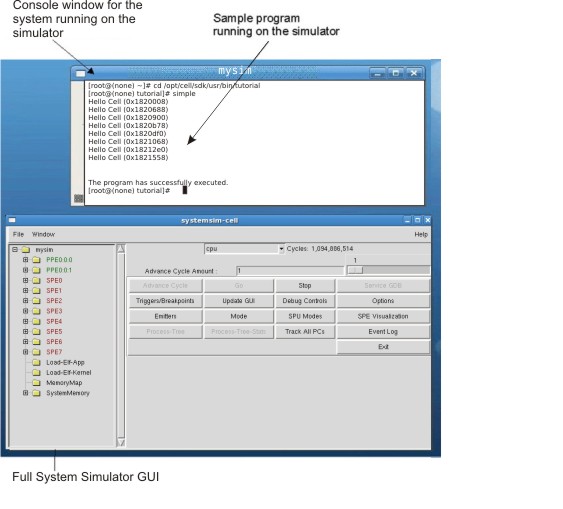
To verify that the simulator is operating correctly and then run it, issue the following commands:
export PATH=/opt/ibm/systemsim-cell/bin:$PATH
systemsim -g
The systemsim script found in the simulator's bin directory launches the simulator. The -g parameter starts the graphical user interface.
When the GUI is displayed, click Go to start the simulator.
You can use the simulator's GUI to get a better understanding of the Cell BE architecture. For example, the simulator shows two sets of PPE state. This is because the PPE processor core is dual-threaded and each thread has its own registers and context. You can also look at the state of the SPE's, including the state of their Memory Flow Controller (MFC).
The systemsim command syntax is:
systemsim [-f file] [-g] [-n]
where:
| Parameter | Description |
|---|---|
| -f <filename> | specifies an initial run script (TCL file) |
| -g | specifies GUI mode, otherwise the simulator starts in command-line mode |
| -n | specifies that the simulator should not open a separate console window |
You can find documentation about the simulator including the user's guide in the /opt/ibm/systemsim-cell/doc directory.
The callthru utility allows you to copy files to or from the simulated system while it is running. The utility is located in the simulator system root image in the /usr/bin directory.
If you call the utility as:
Redirecting appropriately lets you copy files to and from the host. For example, when the simulator is running on the host, you could copy a Cell BE application into /tmp:
cp matrix_mul /tmp
Then, in the console window of the simulated system, you could access it as follows:
callthru source /tmp/matrix_mul > matrix_mul
chmod +x matrix_mul
./matrix_mul
The /tmp directory is shown as an example only.
The source files for the callthru utility are in /opt/ibm/systemsim-cell/sample/callthru. The callthru utility is built and installed onto the sysroot disk as part of the SDK installation process.
By default the simulator does not write changes back to the simulator system root (sysroot) image. This means that the simulator always begins in the same initial state of the sysroot image. When necessary, you can modify the simulator configuration so that any file changes made by the simulated system to the sysroot image are stored in the sysroot disk file so that they are available to subsequent simulator sessions.
To specify that you want update the sysroot image file with any changes made in the simulator session, change the newcow parameter on the mysim bogus disk init command in .systemsim.tcl to rw (specifying read/write access) and remove the last two parameters. The following is the changed line from .systemsim.tcl:
mysim bogus disk init 0 $sysrootfile rw
When running the simulator with read/write access to the sysroot image file, you must ensure that the file system in the sysroot image file is not corrupted by incomplete writes or a premature shutdown of the Linux operating system running in the simulator. In particular, you must be sure that Linux writes any cached data out to the file system before exiting the simulator. To do this, issue "sync ; sync" in the Linux console window just before you exit the simulator.
By default the simulator provides an environment that simulates one Cell BE processor. To simulate an environment where two Cell BE processors exist, similar to a BladeCenter QS21, you must enable Symmetric Multiprocessing (SMP) support. A tcl run script, config_smp.tcl, is provided with the simulator to configure it for SMP simulation. For example, following sequence of commands will start the simulator configured with a graphical user interface and SMP.
export PATH=$PATH:/opt/ibm/systemsim/bin
systemsim -g -f config_smp.tcl
When the simulator is started, it has access to sixteen SPEs across two Cell BE processors.
To enable xclients from the simulator, you need to configure BogusNet (see the BogusNet HowTo), and then perform the following configuration steps:
echo 1 > /proc/sys/net/ipv4/ip_forward
iptables -t nat -A POSTROUTING -o eth0 -j MASQUERADE
iptables -A FORWARD -i eth0 -o tap0 -m state --state RELATED,ESTABLISHED -j ACCEPT
iptables -A FORWARD -i tap0 -o eth0 -j ACCEPT
Many of the tools provided in SDK 3.0 support multiple implementations of the CBEA. These include the Cell BE processor and a future processor. This future processor is a CBEA-compliant processor with a fully pipelined, enhanced double precision SPU.
The processor supports five optional instructions to the SPU Instruction Set Architecture. These include:
Detailed documentation for these instructions is provided in version 1.2 (or later) of the Synergistic Processor Unit Instruction Set Architecture specification. The future processor also supports improved issue and latency for all double precision instructions.
The SDK compilers support compilation for either the Cell BE processor or the future processor.
| Options | Description |
|---|---|
| -march=<cpu type> | Generate machine code for the SPU architecture specified by the CPU type. Supported CPU types are either cell (default) or celledp, corresponding to the Cell BE processor or future processor, respectively. |
| -mtune=<cpu type> | Schedule instructions according to the pipeline model of the specified CPU type. Supported CPU types are either cell (default) or celledp, corresponding to the Cell BE processor or future processor, respectively. |
| Option | Description |
|---|---|
| -qarch=<cpu type> | Generate machine code for the SPU architecture specified by the CPU type. Supported CPU types are either spu (default) or edp, corresponding to the Cell BE processor or future processor, respectively. |
| -qtune=<cpu type> | Schedule instructions according to the pipeline model of the specified CPU type. Supported CPU types are either spu (default) or edp, corresponding to the Cell BE processor or future processor, respectively. |
The simulator also supports simulation of the future processor. The simulator installation provides a tcl run script to configure it for such simulation. For example, the following sequence of commands start the simulator configured for the future processor with a graphical user interface.
export PATH=$PATH:/opt/ibm/systemsim-cell/bin
systemsim -g -f config_edp_smp.tcl
The static timing analysis tool, spu_timing, also supports multiple processor implementations. The command line option -march=celledp can be used to specify that the timing analysis be done corresponding to the future processors' enhanced pipeline model. If the architecture is unspecified or invoked with the command line option -march=cell, then analysis is done corresponding to the Cell BE processor's pipeline model.
When you develop SPE programs using the SDK, you may wish to reference variables in the PPE address space from code running on an SPE. This is achieved through an extension to the C language syntax.
It might be desirable to share data in this way between an SPE and the PPE. This extension makes it easier to pass pointers so that you can use the PPE to perform certain functions on behalf of the SPE. You can readily share data between all SPEs through variables in the PPE address space.
The compiler recognizes an address space identifier __ea that can be used as an extra type qualifier like const or volatile in type and variable declarations. You can qualify variable declarations in this way, but not variable definitions.
The following are examples.
/* Variable declared on the PPE side. */
extern __ea int ppe_variable;

/* Can also be used in typedefs. */
typedef __ea int ppe_int;

/* SPE pointer variable pointing to memory in the PPE address space */
__ea int *ppe_pointer;
Pointers in the SPE address space can be cast to pointers in the PPE address space. Doing this transforms an SPE address into an equivalent address in the mapped SPE local store (in the PPE address space). The following is an example.
int x;
__ea int *ppe_pointer_to_x = &x;
These pointer variables can be passed to the PPE process by way of a mailbox and used by PPE code. With this method, you can perform operations in the PPE execution context such as copying memory from one region of the SPE local store to another.
In the same way, these pointers can be converted to and from the two address spaces, as follows:
int *spe_x;
spe_x = (int *) ppe_pointer_to_x;
References to __ea variables cause decreased performance. The implementation performs software caching of these variables, but there are much higher overheads when the variable is accessed for the first time. Modifications to __ea variables is also cached. The writeback of such modifications to PPE address space may be delayed until the cache line is flushed, or the SPU context terminates.
GCC for the SPU provides the following command line options to control the runtime behavior of programs that use the __ea extension. Many of these options specify parameters for the software-managed cache. In combination, these options cause GCC to link your program to a single software-managed cache library that satisfies those options. Table 5 describes these options.
| Option | Description |
|---|---|
| -mea32 | Generate code to access variables in 32-bit PPU objects. The compiler defines a preprocessor macro __EA32__ to allow applications to detect the use of this option. This is the default. |
| -mea64 | Generate code to access variables in 64-bit PPU objects. The compiler defines a preprocessor macro __EA64__ to allow applications to detect the use of this option. |
| -mcache-size=8 | Specify an 8 KB cache size. |
| -mcache-size=16 | Specify an 16 KB cache size. |
| -mcache-size=32 | Specify an 32 KB cache size. |
| -mcache-size=64 | Specify an 64 KB cache size. |
| -mcache-size=128 | Specify an 128 KB cache size. |
| -matomic-updates | Use DMA atomic updates when flushing a cache line back to PPU memory. This is the default. |
-mno-atomic-updates |
This negates the -matomic-updates option. |
Accessing an __ea variable from an SPU program creates a copy of this value in the local storage of the SPU. Subsequent modifications to the value in main storage are not automatically reflected in the copy of the value in local store. It is your responsibility to ensure data coherence for __ea variables that are accessed by both SPE and PPE programs.
A complete example using __ea qualifiers to implement a quick sort algorithm on the SPU accessing PPE memory can be found in the examples/ppe_address_space directory provided by the SDK 3.0 cell-examples tar ball.
Each of the examples and demos has an associated README.txt file. There is also a top-level readme in the /opt/cell/sdk/src directory, which introduces the structure of the example code source tree.
Almost all of the examples run both within the simulator and on the BladeCenter QS21. Some examples include SPU-only programs that can be run on the simulator in standalone mode.
The source code, which is specific to a given Cell BE processor unit type, is in the corresponding subdirectory within a given example's directory:
In /opt/cell/sdk/buildutils there are some top level Makefiles that control the build environment for all of the examples. Most of the directories in the libraries and examples contain a Makefile for that directory and everything below it. All of the examples have their own Makefile but the common definitions are in the top level Makefiles.
The build environment Makefiles are documented in /opt/cell/sdk/buildutils/README_build_env.txt.
Environment variables in the /opt/cell/sdk/buildutils/make.* files are used to determine which compiler is used to build the examples.
The /opt/cell/sdk/buildutils/cellsdk_select_compiler script can be used to switch the compiler. The syntax of this command is:
/opt/cell/sdk/buildutils/cellsdk_select_compiler [xlc | gcc]
where the xlc flag selects the XL C/C++ compiler and the gcc flag selects the GCC compiler. The default, if unspecified, is to compile the examples with the GCC compiler.
After you have selected a particular compiler, that same compiler is used for all future builds, unless it is specifically overwritten by shell environment variables, SPU_COMPILER, PPU_COMPILER, PPU32_COMPILER, or PPU64_COMPILER.
You do not need to build all the example code at once, you can build each program separately. To start from scratch, issue a make clean using the Makefile in the /opt/cell/sdk/src directory or anywhere in the path to a specific library or sample.
If you have performed a make clean at the top level, you need to rebuild the include files and libraries first before you compile anything else. To do this run a make in the src/include and src/lib directories.
This release of the GNU tool chain includes a GCC compiler and utilities that optimize code for the Cell BE processor. These are:
The example below shows the steps required to create the executable program simple which contains SPU code, simple_spu.c, and PPU code, simple.c.
/usr/bin/spu-gcc -g -o simple_spu simple_spu.c
/usr/bin/ppu32-embedspu simple_spu simple_spu simple_spu-embed.o
/usr/bin/ppu32-gcc -g -o simple simple.c simple_spu-embed.o -lspe
/usr/bin/ppu32-gcc -g -o simple simple.c simple_spu -lspe
The SDK supports the huge translation lookaside buffer (TLB) file system, which allows you to reserve 16 MB huge pages of pinned, contiguous memory. This feature is particularly useful for some Cell BE applications that operate on large data sets, such as the FFT16M workload sample.
To configure the BladeCenter QS21 for 20 huge pages (320 MB), run the following commands:
mkdir -p /huge
echo 20 > /proc/sys/vm/nr_hugepages
mount -t hugetlbfs nodev /huge
If you have difficulties configuring adequate huge pages, it could be that the memory is fragmented and you need to reboot.
You can add the command sequence shown above to a startup initialization script, such as /etc/rc.d/rc.sysinit, so that the huge TLB file system is configured during the system boot.
To verify the large memory allocation, run the command cat /proc/meminfo. The output is similar to:
MemTotal:      1010168 kB
MemFree:        155276 kB
. . .

HugePages_Total:    20
HugePages_Free:     20
Hugepagesize:    16384 kB
Huge pages are allocated by invoking mmap of a /huge file of the specified size. For example, the following code sample allocates 32 MB of private huge paged memory :
int fmem;
  char *mem_file = "/huge/myfile.bin";

  fmem = open(mem_file, O_CREAT | O_RDWR, 0755)) == -1) {
  remove(mem_file);

  ptr = mmap(0, 0x2000000, PROT_READ | PROT_WRITE, MAP_PRIVATE, fmem, 0);
mmap succeeds even if there are insufficient huge pages to satisfy the request. On first access to a page that can not be backed by huge TLB file system, the application is "killed". That is, the process is terminated and the message "killed" is emitted. You must be ensure that the number of huge pages requested does not exceed the number available. Furthermore, on a BladeCenter QS20 and BladeCenter QS21 , the huge pages are equally distributed across both Non-Uniform Memory Architecture (NUMA) memory nodes. Applications that restrict memory allocation to a specific node find that the number of available huge pages for the specific node is half of what is reported in /proc/meminfo.
This section documents some best practices in terms of developing applications using the SDK. See also developerWorks articles about programming tips and best practices for writing Cell BE applications at
http://www.ibm.com/developerworks/power/cell/
Multiple users should not update the common simulator sysroot image file by mounting it read-write in the simulator. For shared development environments, the callthru utility (see The callthru utility) can be used to get files in and out of the simulator. Alternatively, users can copy the sysroot image file to their own sandbox area and then mount this version with read/write permissions to make persistent updates to the image.
If multiple users need to run Cell BE applications on a BladeCenter QS21, you need a machine reservation mechanism to reduce collisions between two people who are using SPEs at the same time. This is because SPE threads are not fully preemptable in this version of the SDK.
The following sections discusses the following performance considerations that you should take into account when you are developing applications:
The BladeCenter QS20 and BladeCenter QS21 are both Non-Uniform Memory Architecture (NUMA) systems, which consist of two Cell BE processors, each with its own system memory. The two processors are interconnected thru a FlexIO interface using the fully coherent BIF protocol. The bandwidth between processor elements or processor elements and memory is greater if accesses are local and do not have to communicate across the FlexIO. In addition, the access latency is slightly higher on node 1 (Cell BE 1) as compared to node 0 (Cell BE 0) regardless of whether they are local or non-local.
To maximize the performance of a single application, you can specify CPU and memory binding to either reduce FlexIO traffic or exploit the aggregated bandwidth of the memory available on both nodes. You can specify the Linux scheduling policy or memory placement either through application-specified NUMA policy library calls (man numa(3)) or using the numactl command (man numactl(8)).
For example, the following command invokes a program that allocates all CPUs on node 0 with a preferred memory allocation on node 0:
numactl --cpunodebind=0 --preferred=0 <program name>
Choosing an optimal NUMA policy depends upon the application's communication and data access patterns. However, you should consider the following general guidelines:
The Linux operating system provides preemptive context switching of virtualized SPE contexts that each resemble the functionality provided by a physical SPE, but there are limitations to the degree to which the architected hardware interfaces can be used in a virtualized environment.
In particular, memory mapped I/O on the problem state register area and MFC proxy DMA access can only be used while the SPE context is both running in a thread and not preempted, otherwise the thread trying to perform these operations blocks until the conditions are met.
This can result in poor performance and deadlocks for programs that over-commit SPEs and rely on SPE thread communications and synchronization. In this case, you should avoid running more SPE threads then there are physical SPEs.
This section describes how to debug Cell BE applications. It describes the following:
GDB is the standard command-line debugger available as part of the GNU development environment. GDB has been modified to allow debugging in a Cell BE processor environment and this section describes how to debug Cell BE software using the new and extended features of the GDBs which are supplied with SDK 3.0.
Debugging in a Cell BE processor environment is different from debugging in a multithreaded environment, because threads can run either on the PPE or on the SPE.
There are three versions of GDB which can be installed on a BladeCenter QS21:
This section also describes how to run applications under gdbserver. The gdbserver program allows remote debugging.
The GDB program released with SDK 3.0 replaces previous versions and contains the following enhancements:
The linker embeds all the symbolic and additional information required for the SPE binary within the PPE binary so it is available for the debugger to access when the program runs. You should use the -g option when compiling both SPE and PPE code with GCC or XLC. W The -g option adds debugging information to the binary which then enables GDB to lookup symbols and show the symbolic information. When you use the toplevel Makefiles of the SDK, you can specify the -g option on compilation commands by setting the CC_OPT_LEVEL makefile variable to -g.
When you use the top level Makefiles of the SDK, you can specify the -g option on compilation by setting the CC_OPT_LEVEL Makefile variable to -g.
For more information about compiling with GCC, see Compiling and linking with the GNU tool chain.
This section assumes that you are familiar with the standard features of GDB. It describes the following topics:
There are several ways to debug programs designed for the Cell BE processor. If you have access to Cell BE hardware, you can debug directly using ppu-gdb . You can also run the application under ppu-gdb inside the simulator. Alternatively, you can debug remotely as described in Setting up remote debugging.
Whichever method you choose, after you have started the application under ppu-gdb, you can use the standard GDB commands available to debug the application. The GDB manual is available at the GNU Web site
http://www.gnu.org/software/gdb/gdb.html
and there are many other resources available on the World Wide Web.
Standalone SPE programs or spulets are self-contained applications that run entirely on the SPE. Use spu-gdb to launch and debug standalone SPE programs in the same way as you use ppu-gdb on PPE programs.
The examples in this section use a standalone SPE (spulet) program, simple.c, whose source code and Makefile are given below:
Source code:
#include <stdio.h>
#include <spu_intrinsics.h>

unsigned int
fibn(unsigned int n)
{
    if (n <= 2)
        return 1;
    return (fibn (n-1) + fibn (n-2));
}

int
main(int argc, char **argv)
{
    unsigned int c;
    c = fibn (8);
    printf ("c=%d\n", c);
    return 0;
}
Makefile:
simple: simple.c
        spu-gcc simple.c -g -o simple
Source-level debugging of SPE programs with spu-gdb is similar in nearly all aspects to source-level debugging for the PPE. For example, you can:
The following example illustrates the backtrace output for the simple.c standalone SPE program.
$ spu-gdb ./simple
GNU gdb 6.7
Copyright (C) 2006 Free Software Foundation, Inc.
GDB is free software, covered by the GNU General Public License, and you are
welcome to change it and/or distribute copies of it under certain conditions.
Type "show copying" to see the conditions.
There is absolutely no warranty for GDB.  Type "show warranty" for details.
This GDB was configured as "--host=powerpc64-unknown-linux-gnu --target=spu"...
(gdb) break 8
Breakpoint 1 at 0x184: file simple.c, line 8.
(gdb) break 18
Breakpoint 2 at 0x220: file simple.c, line 18.
(gdb) run
Starting program: /home/usr/md/fib/simple

Breakpoint 1, fibn (n=2) at simple.c:8
8           return 1;
(gdb) backtrace
#0  fibn (n=2) at simple.c:8
#1  0x000001a0 in fibn (n=3) at simple.c:10
#2  0x000001a0 in fibn (n=4) at simple.c:10
#3  0x000001a0 in fibn (n=5) at simple.c:10
#4  0x000001a0 in fibn (n=6) at simple.c:10
#5  0x000001a0 in fibn (n=7) at simple.c:10
#6  0x000001a0 in fibn (n=8) at simple.c:10
#7  0x0000020c in main (argc=1, argv=0x3ffe0) at simple.c:16
(gdb) delete breakpoint 1
(gdb) continue
Continuing.

Breakpoint 2, main (argc=1, argv=0x3ffe0) at simple.c:18
18        printf("c=%d\n", c);
(gdb) print c
$1 = 21
(gdb)
The spu-gdb program also supports many of the familiar techniques for debugging SPE programs at the assembler code level. For example, you can:
The following example illustrates some of these facilities.
$ spu-gdb ./simple
GNU gdb 6.7
Copyright (C) 2007 Free Software Foundation, Inc.
GDB is free software, covered by the GNU General Public License, and you are
welcome to change it and/or distribute copies of it under certain conditions.
Type "show copying" to see the conditions.
There is absolutely no warranty for GDB.  Type "show warranty" for details.
This GDB was configured as "--host=powerpc64-unknown-linux-gnu --target=spu"...
(gdb) br 18
Breakpoint 1 at 0x220: file simple.c, line 18.
(gdb) r
Starting program: /home/usr/md/fib/simple

Breakpoint 1, main (argc=1, argv=0x3ffe0) at simple.c:18
18        printf("c=%d\n", c);
(gdb) print c
$1 = 21
(gdb) x /8i $pc
0x220 <main+72>:        ila     $3,0x8c0 <_fini+32>
0x224 <main+76>:        lqd     $4,32($1)       # 20
0x228 <main+80>:        brsl    $0,0x2a0 <printf>       # 2a0
0x22c <main+84>:        il      $2,0
0x230 <main+88>:        ori     $3,$2,0
0x234 <main+92>:        ai      $1,$1,80        # 50
0x238 <main+96>:        lqd     $0,16($1)
0x23c <main+100>:       bi      $0
(gdb) nexti
0x00000224      18        printf("c=%d\n", c);
(gdb) nexti
0x00000228      18        printf("c=%d\n", c);
(gdb) print $r4$1 = {uint128 = 0x0003ffd0000000001002002000000030, v2_int64 = {
1125693748412416, 1153484591999221808}, v4_int32 = {262096, 0, 268566560,48},
v8_int16 = {3, -48, 0, 0, 4098, 32, 0, 48},v16_int8 =
"\000\003??\000\000\000\000\020\002\000 \000\000\0000",
v2_double = {5.5616660882883401e-309, 1.4492977868115269e-231},
v4_float = {
3.67274722e-40, 0, 2.56380757e-29, 6.72623263e-44}}
Because each SPE register can hold multiple fixed or floating point values of several different sizes, spu-gdb treats each register as a data structure that can be accessed with multiple formats. The spu-gdb ptype command, illustrated in the following example, shows the mapping used for SPE registers:
(gdb) ptype $r80
type = union __spu_builtin_type_vec128 {
   int128_t uint128;
   int64_t v2_int64[2];
   int32_t v4_int32[4];
   int16_t v8_int16[8];
   int8_t v16_int8[16];
   double v2_double[2];
   float v4_float[4];
}
To display or update a specific vector element in an SPE register, specify the appropriate field in the data structure, as shown in the following example:
(gdb)  p $r80.uint128
$1 = 0x00018ff000018ff000018ff000018ff0
(gdb)  set $r80.v4_int32[2]=0xbaadf00d
(gdb)  p $r80.uint128
$2 = 0x00018ff000018ff0baadf00d00018ff0
SPU local store space is limited. Allocating too much stack space limits space available for code and data. Allocating too little stack space can cause runtime failures. To help you allocate stack space efficiently, the SPU linker provides an estimate of maximum stack usage when it is called with the option --stack-analysis. The value returned by this command is not guaranteed to be accurate because the linker analysis does not include dynamic stack allocation such as that done by the alloca function. The linker also does not handle calls made by function pointers or recursion and other cycles in the call graph. However, even with these limitations, the estimate can still be useful. The linker provides detailed information on stack usage and calls in a linker map file, which can be enabled by passing the parameter -Map <filename> to the linker. This extra information combined with known program behavior can help you to improve on the linker's simple analysis.
For the following simple program, hello.c:
#include <stdio.h>
#include <unistd.h>

int foo (void)
{
   printf (" world\n");
   printf ("brk: %x\n", sbrk(0));
   (void) fgetc (stdin);
   return 0;
}

int main (void)
{
   printf ("Hello");
   return foo ();
}
The command spu-gcc -o hello -O2 -Wl,--stack-analysis,-Map,hello.map hello.c generates the following output:
Stack size for call graph root nodes.
   _start: 0x540
   _fini: 0x40
   call___do_global_dtors_aux: 0x20
   call_frame_dummy: 0x20
   __sfp: 0x0
   __cleanup: 0xc0
   call___do_global_ctors_aux: 0x20
Maximum stack required is 0x540
This output shows that the main entry point _start will require 0x540 bytes of stack space below __stack. There are also a number of other root nodes that the linker fails to connect into the call graph. These are either functions called through function pointers, or unused functions. _fini, registered with atexit() and called from exit, is an example of the former. All other nodes here are unused.
The hello.map section for stack analysis shows:
Stack size for functions. Annotations: '*' max stack, 't' tail call
   _exit: 0x0 0x0
   __call_exitprocs: 0xc0 0xc0
   exit: 0x30 0xf0
      calls:
         _exit
         *  __call_exitprocs
   __errno: 0x0 0x0
   __send_to_ppe: 0x40 0x40
      calls:
         __errno
   __sinit: 0x0 0x0
   fgetc: 0x40 0x80
      calls:
         *  __send_to_ppe
         __sinit
   printf: 0x4c0 0x500
      calls:
         *  __send_to_ppe
   sbrk: 0x20 0x20
      calls:
         __errno
   puts: 0x30 0x70
      calls:
         *  __send_to_ppe
   foo: 0x20 0x520
      calls:
         fgetc
         *  printf
         sbrk
         puts
   main: 0x20 0x520
      calls:
         *t foo
            printf
   __register_exitproc: 0x0 0x0
   atexit: 0x0 0x0
      calls:
         t __register_exitproc
   __do_global_ctors_aux: 0x30 0x30
   frame_dummy: 0x20 0x20
   _init: 0x20 0x50
      calls:
         *  __do_global_ctors_aux
         frame_dummy
   _start: 0x20 0x540
      calls:
         exit
         *  main
         atexit
         _init
   __do_global_dtors_aux: 0x20 0x20
   _fini: 0x20 0x40
      calls:
         *  __do_global_dtors_aux
   call___do_global_dtors_aux: 0x20 0x20
   call_frame_dummy: 0x20 0x20
   __sfp: 0x0 0x0
   fclose: 0x40 0x80
      calls:
         *  __send_to_ppe
         __sinit
   __cleanup: 0x40 0xc0
      calls:
         *  fclose
   call___do_global_ctors_aux: 0x20 0x20
This analysis shows that in the entry for the main function, main requires 0x20 bytes of stack. The total program requires a total of 0x520 bytes including all called functions. The function called from main that requires the maximum amount of stack space is foo, which main calls through thetail function call. Tail calls occur after the local stack for the caller is deallocated. Therefore, the maximum stack space allocated for main is the same as the maximum stack space allocated for foo. The main function also calls the printf function.
If you are uncertain whether the _fini function might require more stack space than main, trace down from the _start function to the __call_exitprocs function (where _fini is called) to find the stack requirement for that code path. The stack size is 0x20 (local stack for _start) plus 0x30 (local stack for exit) plus 0xC0 (local stack for __call_exitprocs) plus 0x40 (total stack for _fini), or 0x150 bytes. Therefore, the stack is sufficient for _fini.
If you pass the --emit-stack-syms option to the linker, it will save the stack sizing information in the executable for use by post-link tools such as FDPRPro. With this option specified, the linker creates symbols of the form __stack_<function_name> for global functions, and __stack_<number>_<function_name> for static functions. The value of these symbols is the total stack size requirement for the corresponding function.
You can link against these symbols. The following is an example.
extern void __stack__start;

   printf ("Total stack is %ld\n", (long) &__stack__start);
The SPE stack shares local storage with the application's code and data. Because local storage is a limited resource and lacks hardware-enabled protection it is possible to overflow the stack and corrupt the program's code or data or both. This often results in hard to debug problems because the effects of the overflow are not likely to be observed immediately.
To understand how to debug stack overflows, it is important to understand how the SPE local storage is allocated and the stack is managed, see Figure 2.
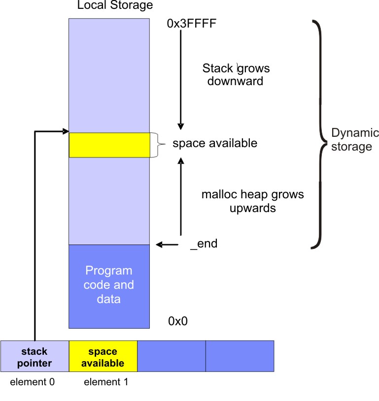
The area between the linker symbol that marks the end of the programs code and data sections, _end, and the top of local storage is dynamic storage. This dynamic storage is used for two purposes, the stack and the malloc heap. The stack grows downward (from high addressed memory to low addressed memory), and the malloc heap grows upward.
The C runtime startup code (crt0) initializes the stack pointer register (register 1) such that word element 0 contains the current stack pointer and word element 1 contains the number of dynamic storage bytes currently available. The stack pointer and space available is negatively adjusted when a stack frame is acquired and positively adjusted when a stack frame is released. The space available is negatively adjusted, up to the available space, whenever the malloc heap is enlarged.
During application development it is advisable that you use stack overflow checking and then disable it when the application is released. Because the spu-gcc and spuxlc compilers do not by default emit code to detect stack overflow, you must include a compile line option:
Stack checking introduces additional code to test for stack overflow. The additional code halts execution conditional on the available space going negative as a result of acquiring or enlarging a stack frame.
For a standalone SPU program, the occurrence of a halt results in a "spe_run: Bad address" message and exit code of SPE_SPU_HALT (4).
For SPE contexts being run from a PPE program, a stack overflow results in a stopinfo, stop_reason of SPE_RUNTIME_ERROR with a spe_runtime_error equal to SPE_SPU_HALT. See the spe_context_run subroutine specification of the SPE Runtime Management Library for additional details.
To reduce the occurrence of stack overflows, you should consider the following strategies:
To debug combined code, that is code containing both PPE and SPE code, you must use ppu-gdb.
Typically a simple program contains only one thread. For example, a PPU "hello world" program is run in a process with a single thread and the GDB attaches to that single thread.
On many operating systems, a single program can have more than one thread. The ppu-gdb program allows you to debug programs with one or more threads. The debugger shows all threads while your program runs, but whenever the debugger runs a debugging command, the user interface shows the single thread involved. This thread is called the current thread. Debugging commands always show program information from the point of view of the current thread. For more information about GDB support for debugging multithreaded programs, see the sections 'Debugging programs with multiple threads' and 'Stopping and starting multi-thread programs' of the GDB User's Manual, available at
http://www.gnu.org/software/gdb/gdb.html
The info threads command displays the set of threads that are active for the program, and the thread command can be used to select the current thread for debugging.
On the Cell BE processor, a thread can run on either the PPE or on an SPE at any given point in time. All threads, both the main thread of execution and secondary threads started using the pthread library, will start execution on the PPE. Execution can switch from the PPE to an SPE when a thread executes the spe_context_run function. See the libspe2 manual for details. Conversely, a thread currently executing on an SPE may switch to use the PPE when executing a library routine that is implemented via the PPE-assisted call mechanism See the Cell BE Linux Reference Implementation ABI document for details. When you choose a thread to debug, the debugger automatically detects the architecture the thread is currently running on. If the thread is currently running on the PPE, the debugger will use the PowerPC architecture. If the thread is currently running on an SPE, the debugger will use the SPE architecture. A thread that is currently executing code on an SPE may also be referred to as an SPE thread.
To see which architecture the debugger is using, use the show architecture command.
Example: show architecture
The example below shows the results of the show architecture command at two different breakpoints in a program. At breakpoint 1 the program is executing in the original PPE thread, where the show architecture command indicates that architecture is powerpc:common. The program then spawns an SPE thread which will execute the SPU code in simple_spu.c. When the debugger detects that the SPE thread has reached breakpoint 3, it switches to this thread and sets the architecture to spu:256K For more information about breakpoint 2, see Setting pending breakpoints.
[user@localhost simple]$ ppu-gdb ./simple
...
...
...
(gdb) break main
Breakpoint 1 at 0x1801654: file simple.c, line 23.
(gdb) run
Starting program: /home/user/md/simple/simple
[Thread debugging using libthread_db enabled]
[New Thread 4160655360 (LWP 2490)]
[Switching to Thread 4160655360 (LWP 2490)]

Breakpoint 1, main (argc=1, argv=0xfff7a9e4) at simple.c:23
23          int i,  status = 0;
(gdb) show architecture
The target architecture is set automatically (currently powerpc:common)
(gdb) break simple_spu.c:5
No source file named simple_spu.c.
Make breakpoint pending on future shared library load? (y or [n]) y

Breakpoint 2 (simple_spu.c:5) pending.
(gdb) continue
Continuing.
Breakpoint 3 at 0x158: file simple_spu.c, line 5.
Pending breakpoint "simple_spu.c:5" resolved
[New Thread 4160390384 (LWP 2495)]
[Switching to Thread 4160390384 (LWP 2495)]

Breakpoint 3, main (id=103079215104) at simple_spu.c:13
13      {
(gdb) show architecture
The target architecture is set automatically (currently spu:256K)
(gdb)
As described in Debugging architecture, any thread of a combined Cell BE application is executing either on the PPE or an SPE at the time the debugger interrupted execution of the process currently being debugged. This determines the main architecture GDB will use when examining the thread. However, during the execution history of that thread, execution may have switched between architectures one or multiple times. When looking at the thread's stack backtrace (using the backtrace command), the debugger will reflect those switches. It will show stack frames belonging to both the PPE and SPE architectures.
Example: An SPE context is interrupted by the debugger while executing a PPE-assisted scanf call
(gdb) backtrace
#0 0x0ff1a8e8 in __read_nocancel () from /lib/libc.so.6
#1 0x0feb7e04 in _IO_new_file_underflow (fp=<value optimized out>) at fileops.c:590
#2 0x0feb82c0 in _IO_default_uflow (fp=<value optimized out>) at genops.c:435
#3 0x0feba518 in *__GI___uflow (fp=<value optimized out>) at genops.c:389
#4 0x0fe9b834 in _IO_vfscanf_internal (s=<value optimized out>, format=<value optimized out>,
argptr=<value optimized out>, errp=<value optimized out>) at vfscanf.c:542
#5 0x0fe9f858 in ___vfscanf (s=<value optimized out>, format=<value optimized out>,
argptr=<value optimized out>)
at vfscanf.c:2473
#6 0x0fe18688 in __do_vfscanf (stream=<value optimized out>, format=<value optimized out>,
vlist=<value optimized out>)
at default_c99_handler.c:284
#7 0x0fe1ab38 in default_c99_handler_vscanf (ls=<value optimized out>, opdata=<value optimized out>)
at default_c99_handler.c:1193
#8 0x0fe176b0 in default_c99_handler (base=<value optimized out>, offset=<value optimized out>)
at default_c99_handler.c:1990
#9 0x0fe1f1b8 in handle_library_callback (spe=<value optimized out>, callnum=<value optimized out>,
npc=<value optimized out>) at lib_builtin.c:152
#10 <cross-architecture call>
#11 0x0003fac4 in ?? ()
#12 0x00000360 in scanf (fmt=<value optimized out>) at ../../../../../../src/newlib/libc/machine/spu/scanf.c:74
#13 0x00000170 in main () at test.c:8
When you choose a particular stack frame to examine using the frame, up, or down commands, the debugger switches its notion of the current architecture as appropriate for the selected frame. For example, if you use the info registers command to look at the selected frame's register contents, the debugger shows the SPE register set if the selected frame belongs to an SPE context, and the PPE register set if the selected frame belongs to PPE code.
Example: continued
gdb) frame 7
#7 0x0fe1ab38 in default_c99_handler_vscanf (ls=<value optimized out>,
opdata=<value optimized out>)
at default_c99_handler.c:1193
1193 default_c99_handler.c: No such file or directory.
in default_c99_handler.c
(gdb) show architecture
The target architecture is set automatically (currently powerpc:common)
(gdb) info registers
r0 0x3 3
r1 0xfec2eda0 4274187680
r2 0xfff9ba0 268409760
r3 0x200 512
<...>

(gdb) frame 13
#13 0x00000170 in main () at test.c:8
8 scanf ("%d\n", &x);
(gdb) show architecture
The target architecture is set automatically (currently spu:256K)
(gdb) info registers
r0 {uint128 = 0x00000170000000000000000000000000, v2_int64 = {0x17000000000, 0x0},
v4_int32 = {0x170, 0x0, 0x0, 0x0}, v8_int16 = {0x0, 0x170, 0x0, 0x0, 0x0, 0x0, 0x0, 0x0},
v16_int8 = {0x0, 0x0, 0x1, 0x70, 0x0 <repeats 12 times>}, v2_double = {0x0, 0x0},
v4_float = {0x0, 0x0, 0x0, 0x0}}
r1 {uint128 = 0x0003ffa0000000000000000000000000, v2_int64 = {0x3ffa000000000, 0x0},
v4_int32 = {0x3ffa0, 0x0, 0x0, 0x0}, v8_int16 = {0x3, 0xffa0, 0x0, 0x0, 0x0, 0x0, 0x0, 0x0},
v16_int8 = {0x0, 0x3, 0xff, 0xa0, 0x0 <repeats 12 times>}, v2_double = {0x0, 0x0},
v4_float = {0x0, 0x0, 0x0, 0x0}}
<...>
Compiling with the '-g' option adds debugging information to the binary that enables GDB to lookup symbols and show the symbolic information.
The debugger sees SPE executable programs as shared libraries. The info sharedlibrary command shows all the shared libraries including the SPE executables when running SPE threads.
Example: info sharedlibrary
The example below shows the results of the info sharedlibrary command at two breakpoints on one thread. At breakpoint 1, the thread is running on the PPE, at breakpoint 3 the thread is running on the SPE. For more information about breakpoint 2, see Setting pending breakpoints.
(gdb) break main
Breakpoint 1 at 0x1801654: file simple.c, line 23.
(gdb) r
Starting program: /home/user/md/simple/simple
[Thread debugging using libthread_db enabled]
[New Thread 4160655360 (LWP 2528)]
[Switching to Thread 4160655360 (LWP 2528)]

Breakpoint 1, main (argc=1, argv=0xffacb9e4) at simple.c:23
23          int i,  status = 0;
(gdb) info sharedlibrary
From        To          Syms Read   Shared Object Library
0x0ffc1980  0x0ffd9af0  Yes         /lib/ld.so.1
0x0fe14b40  0x0fe20a00  Yes         /usr/lib/libspe.so.1
0x0fe5d340  0x0ff78e30  Yes         /lib/libc.so.6
0x0fce47b0  0x0fcf1a40  Yes         /lib/libpthread.so.0
0x0f291cc0  0x0f2970e0  Yes         /lib/librt.so.1
(gdb) break simple_spu.c:5
No source file named simple_spu.c.
Make breakpoint pending on future shared library load? (y or [n]) y

Breakpoint 2 (simple_spu.c:5) pending.
(gdb) c
Continuing.
Breakpoint 3 at 0x158: file simple_spu.c, line 5.
Pending breakpoint "simple_spu.c:5" resolved
[New Thread 4160390384 (LWP 2531)]
[Switching to Thread 4160390384 (LWP 2531)]

Breakpoint 3, main (id=103079215104) at simple_spu.c:13
13      {
(gdb) info sharedlibrary
From        To          Syms Read   Shared Object Library
0x0ffc1980  0x0ffd9af0  Yes         /lib/ld.so.1
0x0fe14b40  0x0fe20a00  Yes         /usr/lib/libspe.so.1
0x0fe5d340  0x0ff78e30  Yes         /lib/libc.so.6
0x0fce47b0  0x0fcf1a40  Yes         /lib/libpthread.so.0
0x0f291cc0  0x0f2970e0  Yes         /lib/librt.so.1
0x00000028  0x00000860  Yes         simple_spu@0x1801d00 <6>
(gdb)
GDB creates a unique name for each shared library entry representing SPE code. That name consists of the SPE executable name, followed by the location in PPE memory where the SPE is mapped (or embedded into the PPE executable image), and the SPE ID of the SPE thread where the code is loaded.
Scheduler-locking is a feature of GDB that simplifies multithread debugging by enabling you to control the behavior of multiple threads when you single-step through a thread. By default scheduler-locking is off, and this is the recommended setting.
In the default mode where scheduler-locking is off, single-stepping through one particular thread does not stop other threads of the application from running, but allows them to continue to execute. This applies to both threads executing on the PPE and on the SPE. This may not always be what you expect or want when debugging multithreaded applications, because those threads executing in the background may affect global application state asynchronously in ways that can make it difficult to reliably reproduce the problem you are debugging. If this is a concern, you can turn scheduler-locking on. In that mode, all other threads remain stopped while you are debugging one particular thread. A third option is to set scheduler-locking to step, which stops other threads while you are single-stepping the current thread, but lets them execute while the current thread is freely running.
However, if scheduler-locking is turned on, there is the potential for deadlocking where one or more threads cannot continue to run. Consider, for example, an application consisting of multiple SPE threads that communicate with each other through a mailbox. If you single-step one thread across an instruction that reads from the mailbox, and that mailbox happens to be empty at the moment, this instruction (and thus the debugging session) will block until another thread writes a message to the mailbox. However, if scheduler-locking is on, that other thread will remain stopped by the debugger because you are single-stepping. In this situation none of the threads can continue, and the whole program stalls indefinitely. This situation cannot occur when scheduler-locking is off, because in that case all other threads continue to run while the first thread is single-stepped. You should ensure that you enable scheduler-locking only for applications where such deadlocks cannot occur.
There are situations where you can safely set scheduler-locking on, but you should do so only when you are sure there are no deadlocks.
The syntax of the command is:
set scheduler-locking <mode>
where mode has one of the following values:
You can check the scheduler-locking mode with the following command:
show scheduler-locking
Generally speaking, you can use the same procedures to debug code for Cell BE as you would for PPC code. However, some existing features of GDB and one new command can help you to debug in the Cell BE processor multithreaded environment. These features are described below.
Breakpoints stop programs running when a certain location is reached. You set breakpoints with the break command, followed by the line number, function name, or exact address in the program.
You can use breakpoints for both PPE and SPE portions of the code. There are some instances, however, where GDB must defer insertion of a breakpoint because the code containing the breakpoint location has not yet been loaded into memory. This occurs when you wish to set the breakpoint for code that is dynamically loaded later in the program. If ppu-gdb cannot find the location of the breakpoint it sets the breakpoint to pending. When the code is loaded, the breakpoint is inserted and the pending breakpoint deleted.
You can use the set breakpoint command to control the behavior of GDB when it determines that the code for a breakpoint location is not loaded into memory. The syntax for this command is:
set breakpoint pending <on off auto>
where
Example: Pending breakpoints
The example below shows the use of pending breakpoints. Breakpoint 1 is a standard breakpoint set for simple.c, line 23. When the breakpoint is reached, the program stops running for debugging. After set breakpoint pending is set to off, GDB cannot set breakpoint 2 (break simple_spu.c:5) and generates the message No source file named simple_spu.c. After set breakpoint pending is changed to auto, GDB sets a pending breakpoint for the location simple_spu.c:5. At the point where GDB can resolve the location, it sets the next breakpoint, breakpoint 3.
(gdb) break main
Breakpoint 1 at 0x1801654: file simple.c, line 23.
(gdb) r
Starting program: /home/user/md/simple/simple
[Thread debugging using libthread_db enabled]
[New Thread 4160655360 (LWP 2651)]
[Switching to Thread 4160655360 (LWP 2651)]

Breakpoint 1, main (argc=1, argv=0xff95f9e4) at simple.c:23
23          int i,  status = 0;
(gdb)  off
(gdb) break simple_spu.c:5
No source file named simple_spu.c.
(gdb) set breakpoint pending auto
(gdb) break simple_spu.c:5
No source file named simple_spu.c.
Make breakpoint pending on future shared library load? (y or [n]) y

Breakpoint 2 (simple_spu.c:5) pending.
(gdb) c
Continuing.
Breakpoint 3 at 0x158: file simple_spu.c, line 5.
Pending breakpoint "simple_spu.c:5" resolved
[New Thread 4160390384 (LWP 2656)]
[Switching to Thread 4160390384 (LWP 2656)]

Breakpoint 3, main (id=103079215104) at simple_spu.c:13
13      {
(gdb)
http://www.gnu.org/software/gdb/gdb.html
The new set spu stop-on-load stops each thread before it starts running on the SPE. While set spu stop-on-load is in effect, the debugger automatically sets a temporary breakpoint on the "main" function of each new SPE thread immediately after it is loaded. You can use the set spu stop-on-load command to do this instead of simply issuing a break main command, because the latter is always interpreted to set a breakpoint on the "main" function of the PPE executable.
The syntax of the command is:
set spu stop-on-load <mode>
where mode is on or off.
To check the status of spu stop-on-load, use the show spu stop-on-load command.
Example: set spu stop-on-load on
(gdb) break main
Breakpoint 1 at 0x1801654: file simple.c, line 23.
(gdb) r
Starting program: /home/user/md/simple/simple
[Thread debugging using libthread_db enabled]
[New Thread 4160655360 (LWP 3009)]
[Switching to Thread 4160655360 (LWP 3009)]

Breakpoint 1, main (argc=1, argv=0xffc7c9e4) at simple.c:23
23          int i,  status = 0;
(gdb) show spu stop-on-load
Stopping for new SPE threads is off.
(gdb) set spu stop-on-load on
(gdb) c
Continuing.
Breakpoint 2 at 0x174: file simple_spu.c, line 16.
[New Thread 4160390384 (LWP 3013)]
Breakpoint 3 at 0x174: file simple_spu.c, line 16.
[Switching to Thread 4160390384 (LWP 3013)]
main (id=25272376) at simple_spu.c:16
16        for (i = 0, n = 0; i<5; i++) {
(gdb) info threads
* 2 Thread 4160390384 (LWP 3013)  main (id=25272376) at simple_spu.c:16
  1 Thread 4160655360 (LWP 3009)  0x0ff27428 in mmap () from /lib/libc.so.6
(gdb) c
Continuing.
Hello Cell (0x181a038) n=3
Hello Cell (0x181a038) n=6
Hello Cell (0x181a038) n=9
Hello Cell (0x181a038) n=12
Hello Cell (0x181a038) n=15
[Thread 4160390384 (LWP 3013) exited]
[New Thread 4151739632 (LWP 3015)]
[Switching to Thread 4151739632 (LWP 3015)]
main (id=25272840) at simple_spu.c:16
16        for (i = 0, n = 0; i<5; i++) {
(gdb) info threads
* 3 Thread 4151739632 (LWP 3015)  main (id=25272840) at simple_spu.c:16
  1 Thread 4160655360 (LWP 3009)  0x0fe14f38 in load_spe_elf (
    handle=0x181a3d8, ld_buffer=0xf6f29000, ld_info=0xffc7c230)
    at elf_loader.c:224
(gdb)
When debugging a combined Cell BE application consisting of a PPE program and more or more SPE programs, it may happen that multiple definitions of a global function or variable with the same name exist. For example, both the PPE and SPE programs will define a global main function. If you run the same SPE executable simultaneously within multiple SPE contexts, all its global symbols will show multiple instances of definition. This might cause problems when attempting to refer to a specific definition from the GDB command line, for example when setting a break point. It is not possible to choose the desired instance of the function or variable definition in all cases.
To catch the most common usage cases, GDB uses the following rules when looking up a global symbol. If the command is issued while currently debugging PPE code, the debugger first attempts to look up a definition in the PPE executable. If none is found, the debugger searches all currently loaded SPE executables and uses the first definition of a symbol with the given name it finds. However, when referring to a global symbol from the command line while currently debugging an SPE context, the debugger first attempts to look up a definition in that SPE context. If none is found there, the debugger continues to search the PPE executable and all other currently loaded SPE executables and uses the first matching definition.
Example:
(gdb) br foo2
Breakpoint 2 at 0x804853f:
file /home/deuling/gdb/dev/gdb/testsuite/gdb.base/solib-symbol-main.c, line 40.

(gdb) delete breakpoints
Delete all breakpoints? (y or n) y

(gdb) br foo
Breakpoint 3 at 0xb7ffd53f:
file /home/deuling/gdb/dev/gdb/testsuite/gdb.base/solib-symbol-lib.c, line 23.

(gdb) continue
Continuing.
Breakpoint 3, foo () at /home/deuling/gdb/dev/gdb/testsuite/gdb.base/solib-symbol-lib.c:23
23 printf ("foo in lib\n");

(gdb) br foo2
Breakpoint 4 at 0xb7ffd569:
file /home/deuling/gdb/dev/gdb/testsuite/gdb.base/solib-symbol-lib.c, line 30.

(gdb) PASS: gdb.base/solib-symbol.exp: foo2 in mdlib
In this example, foo2 is in the main file one time and in the library the other time depending on where GDB currently stands.
In addition to the set spu stop-on-load command, the ppu-gdb and spu-gdb programs offer an extended set of the standard GDB info commands. These are:
If you are working in GDB, you can access help for these new commands. To access help, type help info spu followed by the info spu subcommand name. This displays full documentation. Command name abbreviations are allowed if unambiguous.
http://www.ibm.com/developerworks/power/cell/
Displays SPE event facility status. The output is similar to:
(gdb) info spu event
Event Status 0x00000000
Event Mask   0x00000000
Displays SPE signal notification facility status. The output is similar to:
(gdb) info spu signal
Signal 1 not pending (Type Or)
Signal 2 control word 0x30000001 (Type Or)
Displays SPE mailbox facility status. Only pending entries are shown. Entries are displayed in the order of processing, that is, the first data element in the list is the element that is returned on the next read from the mailbox. The output is similar to:
(gdb) info spu mailbox
SPU Outbound Mailbox
0x00000000
SPU Outbound Interrupt Mailbox
0x00000000
SPU Inbound Mailbox
0x00000000
0x00000000
0x00000000
0x00000000
Displays MFC DMA status. For each pending DMA command, the opcode, tag, and class IDs are shown, followed by the current effective address, local store address, and transfer size (updated as the command is processed). For commands using a DMA list, the local store address and size of the list is shown. The "E" column indicates commands flagged as erroneous by the MFC. The output is similar to:
(gdb) info spu dma
Tag-Group Status  0x00000000
Tag-Group Mask    0x00000000 (no query pending)
Stall-and-Notify  0x00000000
Atomic Cmd Status 0x00000000

Opcode  Tag TId RId EA                 LSA     Size    LstAddr LstSize E
get     1   2   3   0x000000000ffc0001 0x02a80 0x00020                 *
putllc  0   0   0   0xd000000000230080 0x00080 0x00000
get     4   1   1   0x000000000ffc0004 0x02b00 0x00004                 *
mfcsync 0   0   0                      0x00300 0x00880
get     0   0   0   0xd000000000230900 0x00e00 0x00000
0       0   0   0                      0x00000 0x00000
0       0   0   0                      0x00000 0x00000
0       0   0   0                      0x00000 0x00000
0       0   0   0                      0x00000 0x00000
0       0   0   0                      0x00000 0x00000
0       0   0   0                      0x00000 0x00000
0       0   0   0                      0x00000 0x00000
0       0   0   0                      0x00000 0x00000
0       0   0   0                      0x00000 0x00000
0       0   0   0                      0x00000 0x00000
0       0   0   0                      0x00000 0x00000
Displays MFC Proxy-DMA status. The output is similar to:
(gdb) info spu proxydma
Tag-Group Status  0x00000000
Tag-Group Mask    0x00000000 (no query pending)

Opcode  Tag TId RId EA                 LSA     Size    LstAddr LstSize E
getfs   0   0   0   0xc000000000379100 0x00e00 0x00000
get     0   0   0   0xd000000000243000 0x04000 0x00000
0       0   0   0                      0x00000 0x00000
0       0   0   0                      0x00000 0x00000
0       0   0   0                      0x00000 0x00000
0       0   0   0                      0x00000 0x00000
0       0   0   0                      0x00000 0x00000
0       0   0   0                      0x00000 0x00000
There are three versions of gdbserver provided with SDK 3.0:
This section describes how to set up remote debugging for the Cell BE processor and the simulator. It covers the following topics:
You can run an application under gdbserver to allow remote hardware and simulator-based debugging. Gdbserver is a companion program to GDB that implements the GDB remote serial protocol. This is used to convert GDB into a client/server-style application, where gdbserver launches and controls the application on the target platform, and GDB connects to gdbserver to specify debugging commands.
The connection between GDB and gdbserver can either be through a traditional serial line or through TCP/IP. For example, you can run gdbserver on a BladeCenter QS21 and GDB on an Intel(R) x86 platform, which then connects to the gdbserver using TCP/IP.
To use remote debugging, you need a version of the program for the target platform and network connectivity. The gdbserver program comes packaged with GDB and is installed with the SDK 3.0.
When using gdbserver to debug applications on a remote target it is mandatory to provide the same set of libraries (like for example pthread library, C library, libspe, and so on) on both the host (where GDB runs) and the target (where gdbserver runs) system.
Further information on the remote debugging of Cell Broadband Engine applications is available in the DeveloperWorks article at
http://www-128.ibm.com/developerworks/power/library/pa-celldebug/
To start a remote debugging session, do the following:
<gdbserver version> [ip address] :<port> <application> [arg1 arg2 ...]
where
An example for ppu-gdbserver using port 2101 for the program myprog which requires no command line arguments would be:
ppu-gdbserver :2101 myprog
For the simulator this is:
/opt/cell/toolchain/bin/ppu-gdb myprog
For the BladeCenter QS21 this is:
/usr/bin/ppu-gdb myprog
You should have the source and compiled executable version for myprog on the host system. If your program links to dynamic libraries, GDB attempts to locate these when it attaches to the program. If you are cross-debugging, you need to direct GDB to the correct versions of the libraries otherwise it tries to load the libraries from the host platform. The default path is /opt/cell/sysroot. For the SDK 3.0, issue the following GDB command to connect to the server hosting the correct version of the libraries:
set solib-absolute-prefix
target remote 172.20.0.2:2101
where 172.20.0.2 is the IP address of the Cell system that is running gdbserver, and the :2101 parameter is the TCP/IP port parameter that was used start gdbserver. If you are running the client on the same machine then the IP address can be omitted. If you are using the simulator, the IP address is generally fixed at 172.20.0.2 To verify this, enter the ifconfig command in the console window of the simulator.
If gdbserver is running on the simulator, you can use a symbolic host name for the simulator, for example:
target remote systemsim:2101
To do this, edit the host system's /etc/hosts as follows:
# Do not remove the following line, or various programs
# that require network functionality will fail.
127.0.0.1       localhost.localdomain   localhost
172.20.0.2      systemsim
The following shows an example of myprog
   8   {
   9                char *needle, *haystack;
   10                int count = 0;
   11
   12                if (argc < 3) {
   13                    return 0;
   14                }
   15
   16                needle = argv[1];
   17                haystack = argv[2];
   18
B+>19                while (*haystack != '\0')
   20                    {
   21                        int i = 0;
   22                        while (needle[i] != '\0' && haystack[i] != '\0' && needle[i])
   23                            i++
   24                        }
   25                        if (needle[i] == '\0') {
   26                            count++;
   27                        }
   28                        haystack++;
   29                    }
   30
   31                return count;
   32    }
remote Thread 42000 In: main                 Line: 19   PC 0x18004c8
Type "how copying" to see conditions.
There is absolutely no warranty for GDB. Type "show warranty" for details.
This GDB was configured as "--host=i686-pc-linux-gnu --target=powerpc64-linux"....
(gdb) target remote 172.20.0.2:2101
Remote debugging using 172.20.0.2:2101
0xf7ff80f0 in ?? ()
(gdb) b 19
Breakpoint 1 at 0x18004c8: file myprog.c, line 19.
(gdb) c
Continuing.

Breakpoint 1, main (argc=3, argv=0xffab6b74) at myprog.c:19
(gdb)
This section describes the Cell BE Performance Debugging Tool (PDT) and how to configure and enable the tool.
The Cell BE environment enables several levels of parallelism:
Writing applications that utilize such multilevel parallelism effectively, and understanding the performance behavior of such a system, is a challenge. The objective of the Cell BE PDT is to provide programmers with a means of analyzing the execution of such a system and tracking problems in order to optimize execution time and utilization of resources.
This version of the PDT addresses performance debugging of one Cell BE board with two PPEs that share the main memory, run under the same (Linux) operating system, and share up to 16 SPEs. The PDT also enables event tracing on the Hybrid-x86.
Performance analysis is usually based on profiling or tracing. The PDT provides tracing means for recording significant events during program execution and maintaining the sequential order of events. The main objective of the PDT is to provide the ability to trace events of interest, in real time, and record relevant data from the SPEs and PPE. This objective is achieved by instrumenting the code that implements key functions of the events on the SPEs and PPE and collecting the trace records. This instrumentation requires additional communication between the SPEs and PPE as trace records are collected in the PPE memory. Tracing 16 SPEs using one central PPE might lead to a heavy load on the PPE, and therefore, might influence the application performance. The PDT is designed to reduce the tracing execution load and provide a means for throttling the tracing activity on the PPE and each SPE. In addition, the SPE tracing code size is minimized so that it fits into the small SPE local store.
Tracing is enabled at the application level (user space). After the application has been enabled, the tracing facility trace data is gathered every time the application is running.
The Cell BE PDT package is comprised of a tracing facility and a trace analyzer (TA) which is part of the Visual Performance Analyzer (VPA) tool. In addition to the TA, other tools may process and analyze the trace files generated by the tracing facility. The SDK includes the PDT trace Reader/post-processor (PDTR) tool that provides trace-event listings and various summary reports, including lock analysis.
Events tracing is enabled by instrumenting selected function of the following SDK libraries:
Performance events are captured by the SDK functions that are already instrumented for tracing. These functions include; SPEs activation, DMA transfers, synchronization, signaling, user-defined events, etc. Statically linked applications should be compiled and linked with the trace-enabled libraries. Applications using shared libraries are not required to be rebuilt.
Prior to each application run, the user can configure the PDT to trace events of interest. The user can also use the PDT API to dynamically control the tracing.
During the application run, the PPE and SPE trace records are gathered in a memory-mapped (mmap) file in the PPE memory. These records are written into the file system when appropriate. The event-records order is maintained in this file. The SPEs use efficient DMA transfers to write the trace records into the mmap file. The trace records are written in the trace file using a format that is set by an external definition (using an XML file). The PDTR and TA tools, that use PDT traces as input, use the same format definition for visualization and analysis.
The TA processes the trace for analysis and visualization. This processing involves generation of interval records from some of the event records in the trace (e.g., SPE thread life intervals, wait intervals, etc.) as well as adding context parameters (e.g., estimated wall clock time, unique SPE thread ids, etc.) to individual records.
The SDK also provides the PDTR Lock Analyzer program. This command-line tool runs natively on cell and is provided for the viewing and postprocessing of PDT traces (which enables local PDT trace analysis). The PDTR tool provides both sequential and event-by-event PDT trace text output. It also provides postprocessing summary reports based on specific instrumentation events.
Traces can be viewed with the Eclipse-based VPA tool using the Trace Analyzer perspective. This tool provides a means for graphical and textual visualization of trace events over time. It enables programmers to view the details that have been recorded in the trace for each event.
The graphical timeline view in the trace visualization has time as the x axis and the PPE and SPEs as rows in the y axis. Each event interval is shown as a colored bar whose width represents its time duration. The colors in the color legend determine the type of event interval. Figure 3 is a snapshot of the TA GUI on the FFT16M workload.
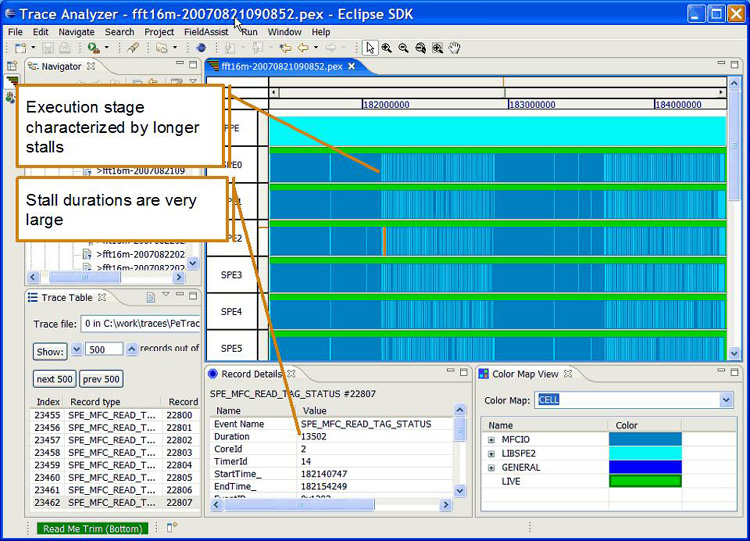
The textual trace overview lists all the PPE and SPE events in order of appearance in the trace. Selecting any event will highlight it in the graphical timeline view and show the fields of the event record in the record details view.
For additional information about trace visualization, refer to the IBM Visual Performance Analyzer User Guide available from IBM alphaWorks:
http://www.alphaworks.ibm.com/tech/vpa
The tracing-facility package is part of the SDK 3.0. Use Table 6 and Table 7 to locate the directories for the tracing-facility package.
| Use | Cell Host |
|---|---|
| Cell BE SDK Development Trace Includes | /usr/include/trace |
| Cell BE SDK Production Trace Libraries | /usr/lib/trace |
| Cell BE SDK Production Trace 64 bits Libraries | /usr/lib64/trace |
| Cell BE SDK SPU Development Trace Includes | /usr/spu/include/trace |
| Cell BE SDK SPU Development Trace Libraries | /usr/spu/lib/trace |
| Use | Cross x86 to Cell |
|---|---|
| Cell BE SDK Development Trace Includes | /opt/cell/sysroot/usr/include/trace |
| Cell BE SDK Production Trace Libraries | /opt/cell/sysroot/usr/lib/trace |
| Cell BE SDK Production Trace 64 bits Libraries | /opt/cell/sysroot/usr/lib64/trace |
| Cell BE SDK SPU Development Trace Includes | /opt/cell/sysroot/usr/spu/include/trace |
| Cell BE SDK SPU Development Trace Libraries | /opt/cell/sysroot/usr/spu/lib/trace |
| Type of file | File path |
|---|---|
| PDT configuration | /usr/share/pdt/config |
| PDT example | /usr/share/pdt/example |
| PDT README | /usr/share/pdt/doc |
The PDT kernel module is a Linux-extension-kernel module that allows the PDT to be synchronized with the Linux SPE context switches. The kernel module is compiled and linked in the pdt.ko file, and is shipped in the /usr/lib/modules/ directory.
The PDT kernel module is loaded by the application before the tracing starts, and removed when the application ends. Since module insertion and removal require su permissions, this operation requires the sudo facility. The call to the sudo facility is integrated within the PDT. To install the facility, update the sudoers line as follows:
ALL ALL=(ALL) NOPASSWD: /sbin/insmod/usr/lib/modules/pdt.ko,/sbin/rmmod_pdt
The PDT package contains a sample application in the /usr/share/pdt/example directory. After installation, the user is advised to compile and run the application, and then examine the PDT output using the TA and PDTR tools.
The example directory contains a Makefile that can be used as a reference. It also contains a sample configuration file. A set of full-reference-configuration files (like pdt_cbe_configuration.xml) is provided in the /usr/share/pdt/config directory. These configuration files can be copied to the user directories and modified as needed.
The PDT tracing facility is designed to minimize the effort that is needed to enable the tracing facility for a given application. In most cases, no code changes or additions are needed. However, because the SPE code is statically linked and the PDT is using a different spu_mfcio.h file, the SPE code must be recompiled. In addition, if the SPE executable is embedded in the PPE code, then the PPE code should be relinked.
Changes to a user's source code are required only if user-defined events or dynamic-trace control is used. For a cross-development environment, root (/) is defined as /opt/cell/sysroot/.
To compile SPE code, do the following:
-Dmain=_pdt_main -Dexit=_pdt_exit -DMFCIO_TRACE -DLIBSYNC_TRACE
To compile PPE code, do the following:
-DLIBSYNC_TRACE
To enable the TA to link between events and the source code, the application should be rebuilt using the linking relocation flags (for SPE and PPE). Use the -Wl and -q flags, but do not use the -s stripping option.
Certain SPU applications, in combination with certain libraries, may present a linking problem when using the PDT. For example, when instrumenting with the PDT, an SPU application that uses a wrapping library (such as ALF), can create a circular dependency. The solution is to specify the trace library twice: once before the wrapping library and once after it. For example:
spu-gcc -o alf_hello_world_spumain_spu.o -L/usr/spu/lib/trace -ltrace -lalf
-L/usr/spu/lib/trace -lsputimer -Wl, -N -ltrace
Another possibility is to use the following option to enable the linker for circular-dependencies search.
-Wl,-\( -lalf -ltrace -Wl,-\)
To run a program using the PDT libraries after the rebuild process, do the following:
The PDT will produce trace files in a directory that is defined by the environment variable PDT_TRACE_OUTPUT. If this environment variable is not defined, the output location is taken from the definition provided by the output_dir attribute in the PDT configuration file. If neither is defined, the current path will be used. The output directory must exist prior to the application run, and the user must have a write access to this directory. The PDT creates the following files in that output directory at each run.
The PDT provides an option to produce events for SPE-programs profiling. The PDTR has an option to produce the profile. To run a program using SPE profiling, do the following:
A configuration XML file is used to configure the PDT. The PDT tracing facility that is built into the application at run time reads the configuration file that is defined by the PDT_CONFIG_FILE environment variable. The /usr/share/pdt/config directory contains a reference configuration file (pdt_cbe_configuration.xml). This file should be copied and then specifically modified for the requirements of each application.
The /usr/share/pdt/config directory also contains reference configuration files for applications that are using the DaCS and ALF libraries: pdt_dacs_config_cell.xml for DaCS and pdt_alf_config_cell.xml for ALF. In addition, a pdt_libsync_config.xml reference file is provided for applications that are using the libsync library.
The first line of the configuration file contains the application name. This name is used as a prefix for the PDT output files. To correlate the output name with a specific run, the name can be changed before each run. The PDT output directory is also defined in the output_dir attribute. This location will be used if the PDT_TRACE_OUTPUT environment variable is not defined.
The first section of the file, <groups>, defines the groups of events for the run. The events of each group are defined in other definition files (which are also in XML format), and included in the configuration file. These files reside in the /usr/share/pdt/config directory. They are provided with the instrumented library and should not be modified by the programmer. Each of these files contains a list of events with the definition of the trace-record data for each event. Note that some of the events define an interval (with StartTime and EndTime), and some are single events (in which the StartTime is 0 and the EndTime is set to the event time). The names of the trace-record fields are the same as the names defined by the API functions. There are two types of records: one for the PPE and one for the SPE. Each of these record types has a different header that is defined in a separate file: pdt_ppe_event_header.xml for the PPE and pdt_spe_event_header.xml for the SPE.
The SDK provides instrumentation for the following libraries (the events themselves are defined in the XML files):
The second section of the file contains the tracing control definitions for each type of processor. The PDT is made ready for the hybrid environment so each processor has a host, <host>. On each processor, several groups of events can be activated in the group control, <groupControl>. Each group is divided into subgroups, and each subgroup, <subgroup>, has a set of events. Each group, subgroup, and event has an active attribute that can be either true or false. This attribute affects tracing as follows:
It is highly recommended that tracing be enabled only for those events that are of interest. Depending on the number of processors involved, programs might produce events at a high rate. If this scenario occurs, the number of traced events might also be very high.
The tracing API used by the PDT is a generic API. It enables any implementation of a tracing facility: the PDT is only one possible implementation. For example, it is possible to implement a tracing facility that only prints a trace.
The PDT APIs is intended for library developers who need to add the tracing facility to their libraries. Because tracing is done "under the covers," applications programmers need only a subset of the API. This subset provides an interface for user-defined events and dynamic-trace control.
The definitions for the PDT API parameters are located in the trace_basic_defs.h and trace_defs.h files that are located in the /usr/include/trace directory.
This API should be used only if the programmer wishes to create user-defined events records in the trace, or if dynamic trace control is needed (at run time).
Include: trace_user.h
The following API enables the programmer to control which events are traced at run time.
Include: trace_dynamic.h
An extended API is provided for library developers. This API is used to instrument a library with generic tracing code. A library may be assigned with one or more groups of events. Each group ID should be obtained from IBM. This requirement enables the usage of any combination of groups in the same run. The PDT can handle up 256 groups: currently 10 groups are in use. Each group can have up to 64 events.
The following function enables the programmer to initiate the tracing facility.
Include: trace_control.h
The following functions are used to create a single-trace record and a trace record that defines an interval.
The following restrictions apply to using the Cell BE PDT.
The tracing-facility package on the Hybrid-x86 is almost identical to the one used on the PPE. Events tracing is enabled by instrumenting selected function of the DaCS and ALF SDK 3.0. libraries.
| Use | Host x86 |
|---|---|
| Cell BE SDK Development Trace Includes | /usr/include/trace |
| Cell BE SDK Production Trace Libraries | /usr/lib/trace |
| Cell BE SDK Production Trace 64 bits Libraries | /usr/lib64/trace |
The /usr/share/pdt/config directory contains reference configuration files for applications that are using the DaCS and ALF libraries: pdt_dacs_config_hybrid.xml for DaCS and pdt_alf_config_hybrid.xml for ALF.
The instrumented events for the Hybrid-x86 libraries are defined in the following files:
The PDT package contains a sample application in the /usr/share/pdt/example directory. After installation, the user is advised to compile and run the application, and then examine the PDT output using the TA and PDTR tools.
The example directory contains a Makefile that can be used as a reference. It also contains a sample configuration file. A set of full-reference-configuration files (pdt_x86_configuration.xml) is provided in the /usr/share/pdt/config directory. These files can be copied to the user directories and modified as needed.
The trace files that are produced during the application run have the same characteristics as those generated on the PPE.
The PDTR tool (pdtr command) is a command-line tool that provides both viewing and postprocessing of PDT traces on the target (client) machine. To use this tool, you must instrument your application by building with the PDT. After the instrumented application has run and created the trace output files, the pdtr command can be run to show the trace output. For example, given PDT instrumented application output files:
       20070604073422.pex              (the xml trace meta file)
       20070604073422.1.trace          (the binary trace data)
       20070604073422.maps             (/proc/<pid>/maps data)
use the pdtr command to generate text based output for this trace as follows:
pdtr [options] 20070604073422
which produces:
20070604073422.pep
This file contains an output summary report for preselected events (such as mutex locking and DMA). If you use the optional -trc flag, the file will also include a time-stamped event-by-event sequential-trace listing. The following is a partial sequential-output trace.
----- Trace File(s) ------------------------------------------------------------------

 Rec#   TimeStamp    DeltaTime Proc EvID  EventName  Event Parameters ...
---------------------------------------------------------------------------------------
    1    0.000000       0.000ms   PPE

    2    1.035853    1035.853ms   PPE  0200 HEART_BEAT EventID=200  Processor=2 PhysicalID=0 EventCount=1
CallingThread=F53DF4B0 StartTime=101248800FFA0B08 EndTime=BABA597C8E7 ProgramCounter=FF8A788
time_of_day=DBC0600000000

    3    1.045290       9.436ms   PPE  0001 CONTEXT_CREATE EventID=1 Processor=2 PhysicalID=0 EventCount=2
CallingThread=F6F8F4B0  StartTime=F7FA3150F7FA3150 EndTime=BABA599D8AB ProgramCounter=10001C50  gang=0 spe=100202C8
flags=0 run_spu_thread()
  :
  :
   38         98        6.845us   SPE  0302 SPE_MFC_GET  EventID=302  Processor=3 PhysicalID=0 EventCount=2
SPEcontext=100202C8 StartTime=0  EndTime=6D PPEcreateContextEventCount=12 ProgramCounter=1754 ea=6D80  ls=10012680
size=80 tagid=1E tid=0 rid=0 main() lspe=1 Size: 0x80 (128), Tag: 0x1e (30)

   39        111        0.908us   SPE 1202 SPE_MFC_READ_TAG_STATUS  EventID=1202  Processor=3 PhysicalID=0 EventCount=3
SPEcontext=100202C8 StartTime=70 EndTime=7A PPEcreateContextEventCount=12 ProgramCounter=1754 _update_type=2
_current_mask=40000000 tag_status=40000000 main() lspe=1  {DMA done[tag=30,0x1e] rec:38 0.908us 141.0MB/s}

   40        124        0.908us   SPE 0503 SPE_MUTEX_LOCK  EventID=503 Processor=3 PhysicalID=0 EventCount=4
SPEcontext=100202C8 StartTime=7D EndTime=87 PPEcreateContextEventCount=12 ProgramCounter=65C lock=10012580 miss=0
main() lspe=1 lock:mylock
  :
   45        196        0.698us  SPE 0703 SPE_MUTEX_UNLOCK EventID=703 Processor=3 PhysicalID=0 EventCount=9
SPEcontext=100202C8 StartTime=BE EndTime=CF PPEcreateContextEventCount=12 ProgramCounter=880 lock=10012580 main()
lspe=1 lock:mylock rec:40 hold=5.0us
  :
  :
See the PDTR man page for additional output examples and usage details.
The following example shows a lock report summary. This report shows summary information for a single lock, shr_lock (address 0x10012180). It shows the total number of accesses to that lock, the hit and miss counts and ratio, and the minimum, average and maximum hold (after the lock is acquired) and wait (waiting on a miss) times. Following this line are the individual callers of the lock (procedure name, address, and logical SPE (lspe) if from SPE code) and the associated hit, miss, hold, and wait times per caller. The asterisk (*) character indicates each lock that was not explicitly initialized with a mutex_init() call.
======================================================================================================================

     Accesses               Hits           Misses       Hit hold time (uS)   Miss wait time (uS)
 Acount  %Total          Count %Acount  Count %Acount   min,   avg,    max   min,   avg,    max     Name
----------------------------------------------------------------------------------------------------------------------
*   600 (100.0 )           3 (  0.5 )   597 ( 99.5 )    100.8, 184.6, 402.4   13.3, 264.4,  568.0   shr_lock (0x10012180)
                           2 ( 66.7 )   298 ( 49.9 )    100.8, 101.1, 101.5  181.8, 249.7,  383.6   main (0x68c)(lspe=1)
                           1 ( 33.3 )   199 ( 33.3 )    200.7, 201.3, 202.5   13.3, 315.2,  568.0   main (0x68c)(lspe=2)
                           0 (  0.0 )   100 ( 16.8 )      0.0,   0.0,   0.0  205.0, 206.8,  278.5   main (0x68c)(lspe=3)
* - Implicitly initialized locks (used before/without mutex_init)
If SPE profiling events are enabled in the PDT configuration file, these profile events are summarized as follows:
Profile:
========
Total SPE profile samples: 426
lspe:1 context:01015D698
   /home/heisch/pep/pt3/gtst1/spu:0
      231 ( 54.2%) 00668-0068B procA
      110 ( 25.8%) 00690-006B3 procB
       57 ( 13.4%) 006B8-006DB procC
       28 (  6.6%) 006E0-00703 procD
The preceding summary shows that of the 426 total sample events, 231 (spe decrementer based) sample events (54.2% of the total) occurred in procA, 110 (25.8% of the total) occurred in procB, etc.
The SDK provide a means of debugging kernel data related to SPUs through specific crash commands, by using a dumped kernel image. This functionality is based on the use of kdump, and the documentation can be found in the Documentation/kdump/kdump.txt file from the Linux kernel sources.
The solution is composed of two environments:
The production system must be a Cell BE hardware. Otherwise, SPU-specific data that is used by crash is not available in the dump file. The analysis system can be any PowerPC hardware, either 32 or 64-bit.
To make use of the SPU crash commands, you need the following SDK packages:
The kernel-debuginfo package is available for for PPC64 architecture. If the analysis system is a 32-bit system, it must be installed in a PPC64 or Cell BE BladeCenter and the /usr/lib/debug/lib/modules-<version>-<release>/vmlinux file must be copied to the analysis system.
You must install all these packages manually. The package crash-spu-commands installs crash if necessary. The following is an example of how to install the analysis system packages using yum:
yum install crash-spu-commands kernel-debuginfo
For the production system, you can use a package manager such as yum to install the packages kernel, kexec-tools, kernel-kdump and busybox-kdump as follows:
yum install kernel kexec-tools kernel-kdump busybox-kdump
busybox-kdump is an optional package, which is recommended for the production system because it provides a custom initrd that allows to boot a dump capture kernel using the minimum amount of memory required to save a dump file.
The production system runs the kernel image included with the SDK kernel package. The following additional steps are required to configure the production system:
The optional package busybox-kdump provides a custom initrd that runs with 48 MB of reserved memory instead of 128 MB, the minimum amount of reserved memory if default initrd is used. This value can be greater than 200 MB, it depends on how many system services are initialized by the system.
To reserve the memory, add the crashkernel=<X>@32M parameter to the kernel boot, where <X> is the number in megabytes to be reserved. In yaboot.conf, the "append" line for the busybox case looks like this:
append="console=hvc0 root=LABEL=/ crashkernel=48M@32M"
After the system has started with the crashkernel parameter, you need to load the dump capture kernel image to the reserved memory. To do this, use the kexec command from the kexec-tools package, as follows:
# Using busybox (crashkernel=44M@32M):
kexec -p /boot/vmlinux-2.6.22.5-bsckdump \
--initrd=/usr/share/busybox/root_initrd/bin/busybox

# Using default initrd (crashkernel=xM@32M, where x >= 128):
kexec -p /boot/vmlinux-2.6.22.5-bsckdump \
--initrd=/boot/initrd-2.6.22.5-bsckdump.img

# Do not use --append with maxcpus parameter,
# as it is known not to work with Cell/B.E. Architecture.
# Maybe it can be used to change the root partition
# where dump kernel will boot, through root parameter.
After running the above command, any future kernel panic event automatically triggers the boot of the dump capture kernel. You can also trigger the dump capture kernel through the use of the "Magic SysRq key" functionality (press Alt+SysRq+C, or echo 'c' to /proc/sysrq-trigger). You might want to do this to capture kernel dump data in the event of a system hang.
After the dump capture kernel has booted, the only task you need to do is to copy the dump file from /proc/vmcore to a persistent storage media. To avoid problems during the dump capture, it is recommended that you define a place to save the dump, which has a size which is about the amount of memory:
cp /proc/vmcore <vmcore_path>
The SPU-commands extension for crash provides commands that format and show data about the state of SPUs at the time of the system crash or hang.
Two parameters are necessary to run crash successfully, these are the production system kernel image compiled with debug info and the kernel dump file. The first is provided by kernel-debuginfo package, in the /usr/lib/debug/lib/modules/<version>-<release>/ directory. The dump file is provided by the dump capture kernel through /proc/vmcore (see previous section).
The order in which the parameters are invoked is not important. For example:
crash /usr/lib/debug/boot/vmlinux-<version>-<release>
<vmcore_path>
If the above files are consistent with each other (<vmcore_path> is generated by a version <version>-<release> kernel), and a crash prompt is provided.
First of all, it is necessary to load the spufs module symbols. This is done by the following command:
crash> mod -s spufs
To use crash SPU-specific commands, use the extend command to load the spu.so file:
crash> extend /usr/lib/crash/extensions/spu.so
When you load the extension, three SPU-specific commands are made available:
These commands are described in the following paragraphs.
You can use the command spus to see which SPE contexts were running at the time of the system crash as shown in the following example:
crash> spus
NODE 0:
ID        SPUADDR      SPUSTATUS       CTXADDR       CTXSTATE    PID
 0   c000000001fac880   RUNNING   c00000003dcbdd80   RUNNABLE    1524
 1   c000000001faca80   RUNNING   c00000003bf34e00   RUNNABLE    1528
 2   c000000001facc80   RUNNING   c00000003bf30e00   RUNNABLE    1525
 3   c000000001face80   RUNNING   c000000039421d00   RUNNABLE    1533
 4   c00000003ee29080   RUNNING   c00000003dec3e80   RUNNABLE    1534
 5   c00000003ee28e80   RUNNING   c00000003bf32e00   RUNNABLE    1526
 6   c00000003ee28c80   STOPPED   c000000039e5e700    SAVED      1522
 7   c00000003ee2e080   RUNNING   c00000003dec4e80   RUNNABLE    1538

NODE 1:
ID        SPUADDR      SPUSTATUS       CTXADDR       CTXSTATE    PID
 8   c00000003ee2de80   RUNNING   c00000003dcbed80   RUNNABLE    1529
 9   c00000003ee2dc80   RUNNING   c00000003bf39e00   RUNNABLE    1535
10   c00000003ee2da80   RUNNING   c00000003bf3be00   RUNNABLE    1521
11   c000000001fad080   RUNNING   c000000039420d00   RUNNABLE    1532
12   c000000001fad280   RUNNING   c00000003bf3ee00   RUNNABLE    1536
13   c000000001fad480   RUNNING   c00000003dec2e80   RUNNABLE    1539
14   c000000001fad680   RUNNING   c00000003bf3ce00   RUNNABLE    1537
15   c000000001fad880   RUNNING   c00000003dec6e80   RUNNABLE    1540
The command spuctx shows context information. The command syntax is:
spuctx [ID | PID | ADDR
For example:
crash> spuctx c00000003dcbdd80 1529

Dumping context fields for spu_context c00000003dcbdd80:
  state                   = 0
  prio                    = 120
  local_store             = 0xc000000039055840
  rq                      = 0xc00000003dcbe720
  node                    = 0
  number                  = 0
  pid                     = 1524
  name                    = spe
  slb_replace             = 0x0
  mm                      = 0xc0000000005dd700
  timestamp               = 0x10000566f
  class_0_pending         = 0
  problem                 = 0xd000080080210000
  priv2                   = 0xd000080080230000
  flags                   = 0x0
  saved_mfc_sr1_RW        = 0x3b
  saved_mfc_dar           = 0xd000000000093000
  saved_mfc_dsisr         = 0x0
  saved_spu_runcntl_RW    = 0x1
  saved_spu_status_R      = 0x1
  saved_spu_npc_RW        = 0x0

Dumping context fields for spu_context c00000003dcbed80:
  state                   = 0
  prio                    = 120
  local_store             = 0xc00000003905a840
  rq                      = 0xc00000003dcbf720
  node                    = 1
  number                  = 8
  pid                     = 1529
  name                    = spe
  slb_replace             = 0x0
  mm                      = 0xc0000000005d1300
  timestamp               = 0x10000566f
  class_0_pending         = 0
  problem                 = 0xd000080080690000
  priv2                   = 0xd0000800806b0000
  flags                   = 0x0
  saved_mfc_sr1_RW        = 0x3b
  saved_mfc_dar           = 0xd0000000000f3000
  saved_mfc_dsisr         = 0x0
  saved_spu_runcntl_RW    = 0x1
  saved_spu_status_R      = 0x1
  saved_spu_npc_RW        = 0x0
You can use the command spurq to visualize all the SPU contexts that were on the SPU run-queue
crash> spurq
PRIO[120]:
c000000000fd7380
c00000003bf31e00
c000000039422d00
c00000000181eb80
This section describes FDPR-Pro. It covers the following topics:
The Post-link Optimization for Linux on POWER tool (FDPR-Pro or fdprpro) is a performance tuning utility that reduces the execution time and the real memory utilization of user space application programs. It optimizes the executable image of a program by collecting information on the behavior of the program under a workload. It then creates a new version of that program optimized for that workload. The new program typically runs faster and uses less real memory than the original program.
The fdprpro tool applies advanced optimization techniques to a program. Some aggressive optimizations might produce programs that do not behave as expected. You should test the resulting optimized program with the same test suite used to test the original program. You cannot re-optimize an optimized program by passing it as input to fdprpro.
The post-link optimizer builds an optimized executable program in three distinct phases:
The optimizer creates an instrumented executable program and an empty template profile file. Type the command fdprpro and specify the instrumentation action as follows:
fdprpro -a instr myprog
The instrumentation phase creates an instrumented file and a profile file. The default filename suffix appended to the instrumented file is .instr and the default filename suffix appended to the profile file is .nprof. Therefore, the preceding command would generate the files myprog.instr and myprog.nprof.
The instrumented program is executed with a representative workload and as it runs it updates the profile file.
The optimizer generates the optimized executable program file. You can control the behavior of the optimizer with options specified on the command line. Type the command fdprpro and specify the optimization action, the (same) input program, the profile file, and the desired optimization flags. The following is an example.
$ fdprpro -a opt -f myprog.nprof [<opts> ...] myprog
The default suffix for the output file name is .fdpr. The preceding command creates an optimized file named myprog.fdpr.
An instrumented executable, created in the instrumentation phase and run in the training phase, typically runs several times slower than the original program. This slowdown is caused by the increased execution time required by the instrumentation. Select a lighter workload to reduce training time to a reasonable value, while still fully exercising the desired code areas.
The input to the fdprpro command must be an executable or a shared library (for PPE files) produced by the Linux linker. fdprpro supports 32-bit or 64-bit programs compiled by the GCC or XLC compilers.
Build the executable program with relocation information. To do this, call the linker with the --emit-relocs (or -q) option. Alternatively, pass the -Wl,--emit-relocs (or -Wl,-q) options to the GCC or XLC compiler.
The SDK helps you build sample programs using a make script named make.footer. It compiles and links both the PPE and SPE parts of a program, and includes a predefined set of compiler and linker options. Typically, a user has a simple Makefile that begins with include $(CELL_TOP)/buildutils/make.footer. To preserve relocation information, add the following lines to the Makefile before the include $(CELL_TOP)/buildutils/make.footer line:
LDFLAGS_xlc += -Wl,-q
LDFLAGS_gcc += -Wl,-q
Alternatively, edit the make.footer file are add "-Wl,-q" to the definition of _LDFLAGS
The fdprpro command creates an instrumented file and a profile file. The profile file is populated with profile information while the instrumented program runs with a specified workload.
The instrumented program requires a shared library named libfsprinst32.so for ELF32 programs, or libfdprinst64.so for ELF64 programs. These libraries are placed in the library search path directory during installation.
The default directory for the profile file is the directory containing the instrumented program. To specify a different directory, set the environment variable FDPR_PROF_DIR to the directory containing the profile file.
If you invoke fdprpro with the basic optimization flag -O, it performs code reordering optimization as well as optimization of branch prediction, branch folding, code alignment and removal of redundant NOOP instructions.
To specify higher levels of optimizations, pass one of the flags -O2, -O3, or -O4 to the optimizer. Higher optimization levels perform more aggressive function inlining, DFA (data flow analysis) optimizations, data reordering, and code restructuring such as loop unrolling. These high level optimization flags work well for most applications. You can achieve optimal performance by selecting and testing specific optimizations for your program.
The fdprpro command accepts many options to control optimization. In our tests, the -O3 option consistently gave good performance results. For complete details, see the fdprpro man page.
When the optimizer processes PPE executables, it generates a profile file and an instrumented file. The profile file is filled with counts while the instrumented file runs. In contrast, when the optimizer processes SPE executables, the profile is generated when the instrumented executable runs. Running a PPE/SPE instrumented executable typically generates a number of profiles, one for each SPE image whose thread is executed. This type of profile accumulates the counts of all threads which execute the corresponding image. The SPE instrumented executable generates an SPE profile named <spename>.mprof in the output directory, where <spename> represents the name of the SPE thread. For more information, see Processing PPE/SPE executable files.
If an old profile exists before instrumentation starts, fdprpro accumulates new data into it. In this way you can combine the profiles of multiple workloads. If you do not want to combine profiles, remove the old profile before starting the optimizer.
The instrumented file is 5% to 20% larger than the original file. Because of the limited local store size of the Cell BE architecture, instrumentation might cause SPE memory overflow. If this happens, fdprpro issues an error message and exits. To avoid this problem, the user can use the --ignore-function-list file or -ifl file option. The file referenced by the file parameter contains names of the functions that should not be instrumented and optimized. This results in a reduced instrumented file size. Specify the same -ifl option in both the instrumentation and optimization phases.
By default, fdprpro processes the executable file as a PPE executable or as an SPE executable, depending on its intended target (the intended target is specified inside the executable file). Two modes are available in order to fully process the PPE/SPE hybrid file: integrated mode, and standalone mode.
The integrated mode of operation does not display the details of SPE processing. This interface is convenient for performing full PPE/SPE processing, but flexibility is reduced. To completely process a PPE/SPE file, run the fdprpro command with the -cell (or --cell-supervisor) command-line option. The following is an example.
$ fdprpro -cell -a instr myprog -o myprog.instr
To optimize the program myprog, type the following command.
$ fdprpro -cell -a opt[<opts> ...] myprog -f myprog.nprof -o myprog.fdpr
The option -spedir specifies the directory into which SPE files are extracted, where they are processed, and from where they are encapsulated back into the PPE file. If this option is not specified, a temporary directory is created in the /tmp directory and is deleted if fdprpro exits without error.
In integrated mode, the same optimization options are used when processing the PPE file and when processing each of the SPE files. Full flexibility is available in standalone mode, where you can specify the explicit commands needed to extract the SPE files, process them, and then encapsulate and process the PPE file. The following list shows the details of this mode.
SPE images are extracted from the input program and written as executable files in the specified directory. The following is an example.
$ fdprpro -a extract -spedir mydir myprog
The SPE images are processed one by one. You should place all of the output files into a distinct directory by their original name. The following is an example.
$ fdprpro -a <action> mydir/<spe1> [-f <prof1>] [<opts> ...] -o outdir/<spe1>
$ fdprpro -a <action> mydir/<spe2> [-f <prof2>] [<opts> ...] -o outdir/<spe2>
...
Select either instr or opt for action. Specify the profile file with the -f command line option. If you do not specify this option, the program searches for a default profile file named mydir/<spename>.mprof in the current directory.
The SPE files are encapsulated as a part of the PPE processing. The following is an example. The -spedir option specifies the output SPE directory.
$ fdprpro -a <action> --encapsulate -spedir mydir [<opts> ...] myprog
In addition to creating an optimized or instrumented program, fdprpro produces human-readable output. The following list details the possible output streams of fdprpro.
FDPR-Pro 5.4.0.10 for Linux (CELL)
fdprpro -a opt -O3 li.linux.gcc32.base -o 1.base
> reading_exe ...
> adjusting_exe ...
> analyzing ...
> building_program_infrastructure ...
...
> updating_executable ...
> writing_executable ...
bye.
Specify the --quiet option to suppress this output.
options.group                   active_options
options.optimization            -bf -bp -dp -hr -hrf 0.10 -kr -las -lro
                                -lu 9 -isf 12 -nop -pr -RC -RD -rt 0.00
                                -si -tlo -vro
options.output                  -o 1.base
global.use_try_and_catch:       0
global.profile_info:            not_available

file.input:                     li.linux.gcc32.base
file.output:                    1.base
file.statistics:                1.base.stat
analysis.csects:                     347
analysis.functions:                  343
analysis.constants:                   13
analysis.basic_blocks:              5360
analysis.function_descriptors:         0
analysis.branch_tables:               10
analysis.branch_table_entries:       374
analysis.unknown_basic_units:         17
analysis.traceback_tables:             0
...
The options specified in the optimization group are those enabled by the -O3 option.
You can invoke fdprpro using the GUI of the Eclipse-based Cell BE IDE. A special plugin is integrated to the IDE to enable this feature. See Cell BE IDE documentation for more detailed information.
FDPR-Pro can be used also in cross-development environment available on Linux X86 systems. The same three-phase profile-driven optimization process is used: instrumentation, profile collection (training), and optimization. In addition, the fdprpro commands used during instrumentation and optimization are identical. The difference is in how profile is collected.
Profile collection in native development is achieved by running the instrumented file locally on the host and using the created profile when performing the optimization phase. However, the instrumented file (like the optimized file) can only be executed on a Cell BE-based system. Perform the following steps to collect the profile in a cross-development environment:
Optimally a complete SPU program is loaded into the local storage of the SPU before it is executed. This is the most efficient method of execution. However, when the sum of the code and data lengths of the program exceeds the local storage size it is necessary to use overlays. (For BladeCenter QS20 the storage size is 256 KB.) Overlays may be used in other circumstances; for example performance might be improved if the size of data areas can be increased by moving rarely used functions to overlays.
An overlay is a program segment which is not loaded into SPU local storage before the main program begins to execute, but is instead left in Cell main storage until it is required. When the SPU program calls code in an overlay segment, this segment is transferred to local storage where it can be executed. This transfer will usually overwrite another overlay segment which is not immediately required by the program.
In an overlay structure the local storage is divided into a root segment, which is always in storage, and one or more overlay regions, where overlay segments are loaded when needed. Any given overlay segment will always be loaded into the same region. A region may contain more than one overlay segment, but a segment will never cross a region boundary.
(A segment is the smallest unit which can be loaded as one logical entity during execution. Segments contain program sections such as functions and data areas.)
The overlay feature is supported for Cell SPU programming (but not for PPU programming) on a native BladeCenter QS20 or on the simulator hosted on an x86 or PowerPC machine.
The code size problem can be addressed through the generation of overlays by the linker. Two or more code segments can be mapped to the same physical address in local storage. The linker also generates call stubs and associated tables for overlay management. Instructions to call functions in overlay segments are replaced by branches to these call stubs, which load the function code to be called, if necessary, and then branch to the function.
In most cases all that is needed to convert an ordinary program to an overlay program is the addition of a linker script to structure the module. In the script you specify which segments of the program can be overlaid. The linker then prepares the required segments so that they may be loaded when needed during execution of the program, and also adds supporting code from the overlay manager library.
At execution time when a call is made from an executing segment to another segment the system determines from the overlay tables whether the requested segment is already in local storage. If not this segment is loaded dynamically (this is carried out by a DMA command), and may overlay another segment which had been loaded previously.
When using overlays you must consider the scope of data very carefully. It is a widespread practice to group together code sections and the data sections used by them. If these are located in an overlay region the data can only be used transiently - overlay sections are not 'swapped out' (written back to Cell BE main storage) as on other platforms but are replaced entirely by other overlays.
Ideally all data sections are kept in the root segment which is never overlaid. If the data size is too large for this then sections for transient data may be included in overlay regions, but the implications of this must be carefully considered.
The overlay structure should be considered at the program planning stage, as soon as code sizes can be estimated. The planning needs to include the number of overlay regions that are required; the number of segments which will be overlaid into each region; and the number of functions within each segment. At this stage it is better to overestimate the number of segments required than to underestimate them. It is easier to combine segments later than to break up oversize segments after they are coded.
The structure of an overlay SPU program module depends on the relationships between the segments within the module. Two segments which do not have to be in storage at the same time may share an address range. These segments can be assigned the same load addresses, as they are loaded only when called. For example, segments that handle error conditions or unusual data are used infrequently and need not occupy storage until they are required.
Program sections which are required at any time are grouped into a special segment called the root segment. This segment remains in storage throughout the execution of an program.
Some overlay segments may be called by several other overlay segments. This can be optimized by placing the called and calling segments in separate regions.
To design an overlay structure you should start by identifying the code sections or stubs which receive control at the beginning of execution, and also any code sections which should always remain in storage. These together form the root segment. The rest of the structure is developed by checking the links between the remaining sections and analyzing these to determine which sections can share the same local storage locations at different times during execution.
Because the minimum indivisible code unit is at the function level, the minimum size of the overlay region is the size of the largest overlaid function. If this function is so large that the generated SPU program does not fit in local storage then a warning is issued by the linker. The user must address this problem by splitting the function into one or more smaller functions.
Even with overlays there are limits on how large an SPE executable can become. An infrastructure of manager code, tables, and stubs is required to support overlays and this infrastructure itself cannot reside in an overlay. For a program with s overlay segments in r regions, making cross-segment calls to f functions, this infrastructure requires the following amounts of local storage:
This allows a maximum available code size of about 512 megabytes, split into 4096 overlay sections of 128 kilobytes each. (This assumes a single entry point into each section and no global data segment or stack.)
Except for the local storage memory requirements described above, this design does not impose any limitations on the numbers of overlay segments or regions supported.
Suppose that a program contains seven sections which are labelled SA through SG, and that the total length of these exceeds the amount of local storage available. Before the program is restructured it must be analyzed to find the optimum overlay design.
The relationship between segments can be shown with a tree structure. This graphically shows how segments can use local storage at different times. It does not imply the order of execution (although the root segment is always the first to receive control). Figure 4 shows the tree structure for this program. The structure includes five segments:
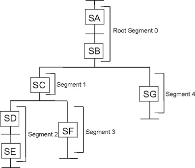
The position of the segments in an overlay tree structure does not imply the sequence in which the segments are executed; in particular sections in the root segment may be called from any segment. A segment can be loaded and overlaid as many times as the logic of the program requires.
For purposes of illustration, assume the sections in the example program have the following lengths:
| Section | Length (in bytes) |
|---|---|
| SA | 30,000 |
| SB | 20,000 |
| SC | 60,000 |
| SD | 40,000 |
| SE | 30,000 |
| SF | 60,000 |
| SG | 80,000 |
If the program did not use overlays it would require 320 KB of local storage; the sum of all sections. With overlays, however, the storage needed for the program is the sum of all overlay regions, where the size of each region is the size of its largest segment. In this structure the maximum is formed by segments 0, 4, and 2; these being the largest segments in regions 0, 1, and 2. The sum of the regions is then 200 KB, as shown in Figure 5.
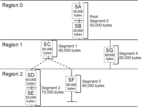
The linker typically assigns the origin of the root segment (the origin of the program) to address 0x80. The relative origin of each segment is determined by the length of all previously defined regions. For example, the origin of segments 2 and 3 is equal to the root origin plus 80 KB (the length of region 1 and segment 4) plus 50 KB (the length of the root segment), or 0x80 plus 130 KB. The origins of all the segments are as follows:
| Segment | Origin |
|---|---|
| 0 | 0x80 + 0 |
| 1 | 0x80 + 50,000 |
| 2 | 0x80 + 130,000 |
| 3 | 0x80 + 130,000 |
| 4 | 0x80 + 50,000 |
The segment origin is also called the load point, because it is the relative location where the segment is loaded. Figure 6 shows the segment origin for each segment and the way storage is used by the example program. The vertical bars indicate segment origin; two segments with the same origin can use the same storage area. This figure also shows that the longest path is that for segments 0, 4, and 2.
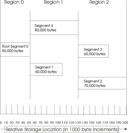
The overlay processing is initiated when a section in local storage calls a section not in storage. The function which determines when an overlay is to occur is the overlay manager. This checks which segment the called section is in and, if necessary, loads the segment. When a segment is loaded it overlays any segment in storage with the same relative origin. No overlay occurs if one sectioncalls another section which is in a segment already in storage (in another region or in the root segment).
The overlay manager uses special stubs and tables to determine when an overlay is necessary. These stubs and tables are generated by the linker and are part of the output program module. The special stubs are used for each inter-segment call. The tables generated are the overlay segment table and the overlay region table. Figure 7 shows the location of the call stubs and the segment and region tables in the root segment in the example program.
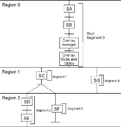
The size of these tables must be considered when planning the use of local storage.
There is one call stub for each function in an overlay segment which is called from a different segment. No call stub is needed if the function is called within the same segment. All call stubs are in the root segment. During execution the call stub specifies (to the overlay manager) the segment to be loaded, and the segment offset to transfer control to, to invoke the function after it is loaded.
Each overlay program contains one overlay segment table and one overlay region table. These tables are in the root segment. The segment table contains static (read-only) information about the relationship of the segments and regions in the program. During execution the region table contains dynamic (read-write) control information such as which segments are loaded into each region.
If the same section is used by several segments it is usually desirable to place that section in the root segment. However, the root segment can get so large that the benefits of overlay are lost. If some of the sections in the root segment could overlay each other then the program might be described as an overlay graph structure (as opposed to an overlay tree structure) and it should use multiple regions.
With multiple regions each segment has access to both the root segment and other overlay segments in other regions. Therefore regions are independent of each other.
Figure 8 shows the relationship between the sections in the example program and two new sections: SH and SI. The two new sections are each used by two other sections in different segments. Placing SH and SI in the root segment makes the root segment larger than necessary, because SH and SI can overlay each other. The two sections cannot be duplicated in two paths, because the linker automatically deletes the duplicates.
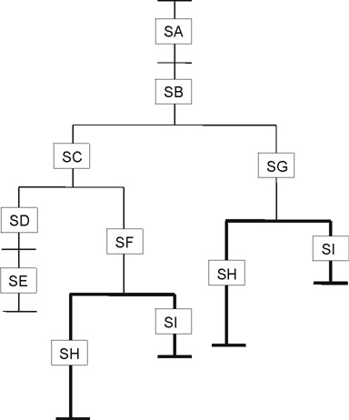
However, if the two sections are placed in another region they can be in local storage when needed, regardless of the segments executed in the other regions. Figure 9 shows the sections in a four-region structure. Either segment in region 3 can be in local storage regardless of the segments being executed in regions 0, 1, or 2. Segments in region 3 can cause segments in region 0, 1 or 2 to be loaded without being overlaid themselves.
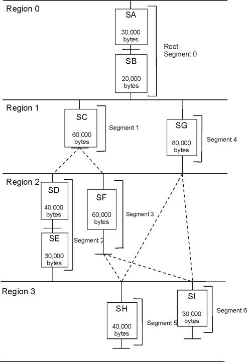
The relative origin of region 3 is determined by the length of the preceding regions (200 KB). Region 3, therefore, begins at the origin plus 200 KB.
The local storage required for the program is determined by adding the lengths of the longest segment in each region. In Figure 9 if SH is 40 KB and SI is 30 KB the storage required is 240 KB plus the storage required by the overlay manager, its call stubs and its overlay tables. Figure 10 shows the segment origin for each segment and the way storage is used by the example program.
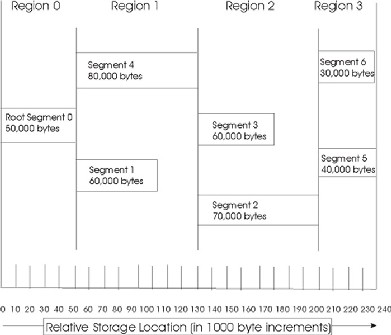
Once you have designed an overlay structure, the program must be arranged into that structure. You must indicate to the linker the relative positions of the segments, the regions, and the sections in each segment, by using OVERLAY statements. Positioning is accomplished as follows:
The input sequence of control statements and sections should reflect the sequence of the segments in the overlay structure (for example the graph in Figure 9), region by region, from top to bottom and from left to right. This sequence is illustrated in later examples.
The origin of every region is specified with an OVERLAY statement. Each OVERLAY statement defines a load point at the end of the previous region. That load point is logically assigned a relative address at the quadword boundary that follows the last byte of the largest segment in the preceding region. Subsequent segments defined in the same region have their origin at the same load point.
In the example overlay tree program, two load points are assigned to the origins of the two OVERLAY statements and their regions, as shown in Figure 4. Segments 1 and 4 are at the first load point; segments 2 and 3 are at the second load point.
The following sequence of linker script statements results in the structure in Figure 5.
OVERLAY {
	.segment1 {./sc.o(.text)}
	.segment4 {./sg.o(.text)}
}
OVERLAY {
	.segment2 {./sd.o(.text) ./se.o(.text)}
	.segment3 {./sf.o(.text)}
}
Note: By implication sections SA and SB are associated with the root segment because they are not specified in the OVERLAY statements.
In the example overlay graph program, as shown in Figure 8, one more load point is assigned to the origin of the last OVERLAY statement and its region. Segments 5 and 6 are at the third load point.
The following linker script statements add to the sequence for the overlay tree program creating the structure shown in Figure 9:
.
.
.
OVERLAY {
	.segment5 {./si.o(.text)}
	.segment6 {./sh.o(.text)}
}
This feature will work with both IPA and non-IPA code, though the partitioning algorithm will generate better overlays with IPA code.
| Option | Description |
|---|---|
| -qipa=overlay | Specifies that the compiler should automatically create code overlays. The -qipa=partition={small|medium|large} option is used to control the size of the overlay buffer. The overlay buffer will be placed after the text segment of the linker script. |
| -qipa=nooverlay | Specifies that the compiler should not automatically create code overlays. This is the default behavior for the dual source compiler. |
| -qipa=overlayproc=<names_list> | Specifies a comma-separated list of functions that should be in the same overlay. Multiple overlayproc suboptions may be present to specify multiple overlay groups. If a procedure is listed in multiple groups, it will be cloned for each group referencing it. C++ function names must be mangled. |
| -qipa=nooverlayproc= <names_list> | Specifies a comma-separated list of functions that should not be overlaid. These will always be resident in the local store. C++ function names must be mangled. |
Examples:
# Compile and link without overlays.
xlc foo.c bar.c
xlc foo.c bar.c -qipa=nooverlay

# Compile and link with automatic overlays.
xlc foo.c bar.c -qipa=overlay

# Compile and link with automatic overlays and ensure that foo and bar are
# in the same overlay. The main function is always resident.
xlc foo.c bar.c -qipa=overlay:overlayproc=foo,bar:nooverlayproc=main

# Compile and link with automatic overlays and a custom linker script.
xlc foo.c bar.c -qipa=overlay -Wl,-Tmyldscript
Three examples are considered:
These examples can be found in the cell-examples RPMs included in the SDK.
This example consists of a single PPU program named driver which creates an SPU thread and launches an embedded SPU main program named spu_main. The SPU program calls four functions: o1_test1, o1_test2, o2_test1, and o2_test2. The first two functions are defined in a single compilation unit, olay1/test.c, and the second two functions are similarly defined in olay2/test.c. See the calling diagram in Figure 11. Upon completion of the SPU thread the driver returns a value from the SPU program to the PPU program.
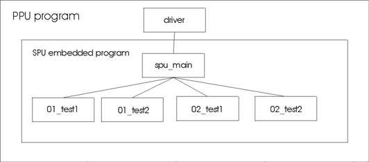
The SPU program is organized as an overlay program with two regions and three segments. The first region is the non-overlay region containing the root segment (segment 0). This root segment contains the spu_main function along with overlay support programming and tables (not shown). The second region is an overlay region and contains segments 1 and 2. In segment 1 are the code sections of functions o1_test1 and o1_test2, and in segment 2 are the code sections of functions o2_test1 and o2_test2, as shown in Figure 12.
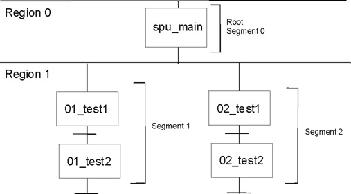
Combining these figures yields the following diagram showing the structure of the SPU program.
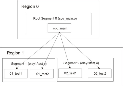
The physical view of this example (Figure 14) shows one region containing the non-overlay root segment, and a second region containing one of two overlay segments. Because the functions in these two overlay segments are quite similar their lengths happen to be the same.
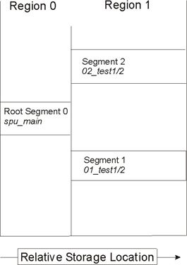
The spu_main program calls its sub-functions multiple times. Specifically the spu_main program first calls two functions, o1_test1 and o1_test2, passing in an integer value (101 and 102 respectively) and upon return it expects an integer result (1 and 2 respectively). Next spu_main calls the two other functions, o2_test1 and o2_test2 passing in an integer value (201 and 202 respectively) and upon return it expects an integer result (11 and 12 respectively). Finally spu_main calls again the first two functions, o1_test1 and o1_test2 passing in an integer value (301 and 302 respectively) and upon return it expects an integer result (1 and 2 respectively). Between each pair of calls, the overlay manager loads the appropriate segment into the appropriate region. In this case, for the first pair it loads segment 1 into region 1 then for the second pair it loads segment 2 into region 1, and for the last pair it reloads segment 1 back into region 1. See Figure 15.
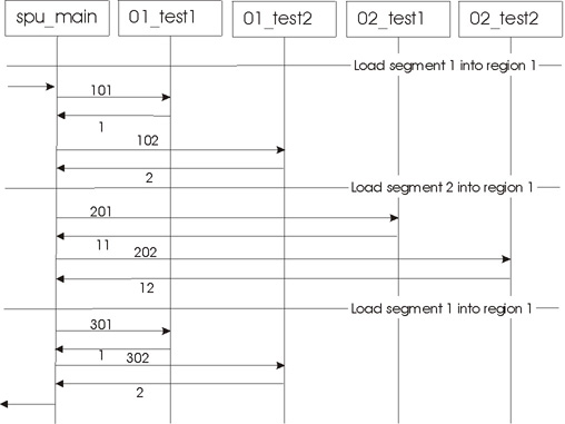
LDFLAGS = -Wl,-T,linker.script
The linker commands are in linker.script.ed which is created in the overlay Makefiles. As part of Makefile processing, this file is converted into the linker.script file used by the linker. In this ed command script the files in the overlay segments are explicitly excluded from the .text non-overlay segment:
/ \.text /
/\*(\.text/
s/\*(\.text/*( EXCLUDE_FILE(olay1\/*.o olay2\/*.o) .text/
/} =0/
a
OVERLAY :
{
.segment1 {olay1/*.o(.text)}
.segment2 {olay2/*.o(.text)}
}
.
w
The overview overlay program is an adaptation of the program described in Overlay graph structure example. The structure is the same as that shown in Figure 9 but the sizes of each segment are different. Each function is defined in its own compilation unit; a distinct file with a name the same as the function name.
The example consists of a single SPU main program. The main program calls the SA function which in turn calls the SB function. These three functions are all located in the root segment (segment 0) and cannot be overlaid.
The SB function calls the SC and SG functions. These are in two segments which are both located in region 1 and overlay each other.
SC calls SD and SF. SD in turn calls SE. The SD and SE functions are in segment 2 and the SF function is in segment 3. These two segments are both located in region 2 and overlay each other.
The SF and SG functions call the SH and SI functions. SI is in segment 6, and SH is in segment 5. These two segments are both located in region 3 and overlay each other.
The physical view of this example (Figure 10) shows the four regions; one region containing a single non-overlay root segment and three regions containing six overlay segments.
LDFLAGS = -Wl,-T,linker.script
The linker commands are in linker.script.ed which is created in the overlay Makefiles.As part of Makefile processing, this file is converted into the linker.script file used by the linker.
:
/ \.text /
/\*(\.text/
s/\*(\.text/*( EXCLUDE_FILE(sc.o sg.o sd.o sf.o sh.o si.o) .text/
/} =0/
a
OVERLAY :
{
.segment1 {sc.o(.text)}
.segment4 {sg.o(.text) }
}
OVERLAY :
{
.segment2 {sd.o(.text) se.o(.text)}
.segment3 {sf.o(.text)}
}
OVERLAY :
{
.segment5 {sh.o(.text)}
.segment6 {si.o(.text)}
}
.
w
The large matrix overlay program consists of a single monolithic non-overlay SPU standalone program. This new example takes the existing program and converts it to an overlay program by providing a linker script. No changes (such as re-compilation) are made to the current library or to the test case code.
The updated example consists of a single standalone SPU program, large_matrix, which calls test functions test_index_max_abs_vec and test_solve_linear_system amongst others. These functions are defined in the single compilation unit large_matrix.c. A simplified structure is shown in Figure 16 (some functions, and some calls within a region, have been omitted for clarity). If the test completes successfully the function returns a zero value; in other cases it returns a non-zero value.
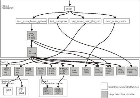
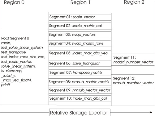
The physical view of this example in Figure 17 shows three regions; one containing a single non-overlay root segment, and two containing twelve overlay segments.
This assumes the archive library directory, /opt/cell/sdk/usr/lib, and the archive library, liblarge_matrix.a, are specified to the SPU linker.
LDFLAGS = -Wl,-T,linker.script
The linker commands are in linker.script.ed which is created in the overlay Makefiles.As part of Makefile processing, this file is converted into the linker.script file used by the linker.
The ed command linker script is:
/ \.text /
/\*(\.text/
s/\*(\.text/*( EXCLUDE_FILE(scale_vector.o* scale_matrix_col.o* swap_vectors.o*
swap_matrix_rows.o* index_max_abs_vec.o* solve_triangular.o* transpose_matrix.o*
nmsub_matrix_matrix.o* nmsub_vector_vector.o* index_max_abs_col.o* madd_number_vector.o*
nmsub_number_vector.o*) .text/
/} =0/
a
OVERLAY :
{
.segment01 {scale_vector.o*(.text)}
.segment02 {scale_matrix_col.o*(.text)}
.segment03 {swap_vectors.o*(.text)}
.segment04 {swap_matrix_rows.o*(.text)}
.segment05 {index_max_abs_vec.o*(.text)}
.segment06 {solve_triangular.o*(.text)}
.segment07 {transpose_matrix.o*(.text)}
.segment08 {nmsub_matrix_matrix.o*(.text)}
.segment09 {nmsub_vector_vector.o*(.text)}
.segment10 {index_max_abs_col.o*(.text)}
}
OVERLAY :
{
.segment11 {madd_number_vector.o*(.text)}
.segment12 {nmsub_number_vector.o*(.text)}
}
.
w
The GNU SPU linker takes object files, object libraries, linker scripts, and command line options as its inputs and produces a fully or partially linked object file as its output. It is natural to control generation of overlays via a linker script as this allows maximum flexibility in specifying overlay regions and in mapping input files and functions to overlay segments. The linker has been enhanced so that one or more overlay regions may be created by simply inserting multiple OVERLAY statements in a standard script; no modification of the subsequent output section specifications, such as setting the load address, is necessary. (It is also possible to generate overlay regions without using OVERLAY statements by defining loadable output sections with overlapping virtual memory address (VMA) ranges.)
On detection of overlays the linker automatically generates the data structures used to manage them, and scans all non-debug relocations for calls to addresses which map to overlay segments. Any such call, apart from those used in branch instructions within the same section, causes the linker to generate an overlay call stub for that address and to remap the call to branch to that stub. At execution time these stubs call an overlay manager function which loads the overlay segment into storage, if necessary, before branching to the final destination.
If the linker command option: -extra-overlay-stubs is specified then the linker generates call stubs for all calls within an overlay segment, even if the target does not lie within an overlay segment (for example if it is in the root segment). Note that a non-branch instruction referencing a function symbol in the same section will also cause a stub to be generated; this ensures that function addresses which escape via pointers are always remapped to a stub as well.
The management data structures generated include two overlay tables in a .ovtab section. The first of these is a table with one entry per overlay segment. This table is read-only to the overlay manager, and should never change during execution of the program. It has the format:
struct {
  u32 vma;    // SPU local store address that the section is loaded to.
  u32 size;   // Size of the overlay in bytes.
  u32 offset; // Offset in SPE executable where the section can be found.
  u32 buf;    // One-origin index into the _ovly_buf_table.
} _ovly_table[];
The second table has one entry per overlay region. This table is read-write to the overlay manager, and changes to reflect the current overlay mapping state. The format is:
struct {
  u32 mapped; // One-origin index into _ovly_table for the
              // currently loaded overlay. 0 if none.
} _ovly_buf_table[];
Whenever the overlay manager loads an segment into a region it updates the mapped field in the _ovly_buf_table entry for the region with the index of the segment entry in the _ovly_buf table.
The overlay manager may be provided by the user as a library containing the entries __ovly_load and _ovly_debug_event. (It is an error for the user to provide _ovly_debug_event without also providing __ovly_load.) If these entries are not provided the linker will use a built-in overlay manager which contains these symbols in the .stub section.
This section provides a summary of the changes to SDK 3.0 from previous versions. It is particularly useful if you have been working with SDK 2.1 and plan to upgrade to SDK 3.0-
There are several changes in the placement of code and libraries compared to previous SDKs:
The following is a list of the SDK 3.0 packages:
The following have been removed:
If you have code that needs these files and does not compile in the SDK 3.0 environment, you need to add the proper #include to your source files.
The function for compiler selection has been removed from the cellsdk script and exists in a new user-level script named cellsdk_select_compiler. The script accepts a single parameter that may be either "gcc" or "xlc".
The make.env file that is modified by this script defaults to GCC, so this command only needs to be run to select the XLC compiler.
The function to synchronize the simulator sysroot image has been removed from the cellsdk script and exists in a new user-level script named cellsdk_sync_simulator.
This script mounts the simulator sysroot image at /mnt/cell-sdk-sysroot and copies files from the platform sysroot to the Simulator sysroot image. For Cell BE platforms the sysroot is / and for non-Cell BE platforms it is /opt/cell/sysroot.
If the install parameter is provided, then RPMs stored in the /tmp/cellsdk/rpms directory are copied into the simulator sysroot image and installed into the simulator using a custom TCL script. The script removes the RPMs, so if you need them again, you should copy them to a location different from /tmp/cellsdk/rpms.
This section describes known issues that you may encounter and suggested solutions.
Symptoms: when running the user application (with PDT enabled) the following message appears: "(PDT) ERROR: Environment variable PDT_CONFIG_FILE was not set."
Solution: Set PDT_CONFIG_FILE to the right PDT configuration file.
Symptoms: when running the user application (with PDT enabled) one of the following happen: a. Bus error: likely when a SPU starts running (when spe_context_run is called). b. Message: "error while loading shared libraries: libtrace.so.3: cannot open shared object file: No such file or directory".
Solution: In both cases, the LD_LIBRARY_PATH is not set, incorrectly set (wrong path or 32/64 path error), or the paths' order is wrong where the PDT library path appears (/usr/lib[64]/trace) after another path so another library occlude the PDT library.
Symptoms: No context switch notifications records exist in the output trace files
Solution: Verify that the PDT kernel module is installed. Verify that the PDT_KERNEL_MODULE environment variable is set to the correct directory files (generally should be set to /usr/lib/modules/pdt.ko).
Symptoms: the following messages are related:
Solution: for 1, 2, 3, 4, and 5, the respective throttling sections of the config file should be checked. Problems 6, 7, and 8 mean that the value of the PDT_CONFIG_FILE environment variable is wrong (e.g. the file doesn't exists, it is not an XML config file, the file is corrupted, the value is a directory instead a config file, etc.). Finally, 9 and 10, mean that the "<configuration name="PROCESSOR">" tag in the config file is missing or an unknown processor for PDT.
Symptoms: Cannot compile/link the PPU program with PDT libraries.
Solution: Recompilation of the PPE code is needed when user events or dynamic control were added to the code, and relinking is needed when compilation is needed or the SPU code is embedded in the PPE executable. Make sure that "-I[/opt/cell/sysroot]/usr/include/trace" flag is used for compilation and "-ltrace" and "-L[/opt/cell/sysroot]/usr/lib[64]/trace" are used for linkage.
Symptoms: The program terminates with bus error or segmentation fault when starting the SPE program run.
Solution: First, check that the LD_LIBRARY_PATH is defined correctly (see problem "Missing/wrong LD_LIBRARY_PATH environment variable at runtime"). Check that the SPE was compiled with PDT, specially look for the -Dmain=_pdt_main flag. If this is not the problem, recompile the SPE code with -Os (optimization for shorter code), in order to verify that PDT code in the SPE executable does not grow the executable to a size bigger than the 256K size allowed.
Symptoms: In the output trace files, there are some context switch notifications with an unknown thread ID value.
Solution: Do not relate to this context switches. Also, make sure that the SPEs are running before trying to access their problem state (e.g. send a mailbox, etc). In addition, only one user can use PDT at a time.
Symptoms: "warning: implicit declaration of function 'trace_XXXXX' ".
Solution: The trace_* functions were added to the code but their respective "#include" are missing. (It is possible that the name of the function is wrong, too).
Symptoms: Undesired events are recorded, or, desired events are not recorded.
Solution: Check the XML configuration file pointed by the PDT_CONFIGURATION_FILE environment variable.
Symptoms: spu_mfcio (SPU) events are not recorded in the trace file.
Solution: Make sure that the flag "-DMFCIO_TRACE" is in the compilation of ALL the SPE files. Also make sure that the flag "-I[/opt/cell/sysroot]/usr/spu/include/trace" appears as the first include flag ("-I") in the compilation command.
Symptoms: The trace shows large intervals in many SPEs and PPE at the same time.
Solution: If the intervals durations are intersected by a "DAEMON interval", then PDT was halted for some milliseconds by the OS. The user should not relate to these large intervals as a problem in the user's code.
Symptoms: No trace files in the expected directory.
Solution: Check if the PDT_TRACE_OUTPUT is defined and see if the files were not written there. If the environment variable wasn't defined, check the output directory that is defined in the configuration file and see if the files were not written there. Check that the directory exists and that write permission is granted for the current user. Note that if both are not defined the trace output is directed to the current directory.
Symptoms: Many trace files are written to the disk and the program fails with error.
Solution: Check space in the hard disk. Try using static or dynamic throttling to decrease the amount of events written to the trace files.
Symptoms: When linking the PPE code,"-ltrace" and "-L/usr/lib[64]/trace" should be added, and then the message "undefined reference to `_Unwind_GetIPInfo@GCC_4.2.0'" shows up.
Solution: add also "-lstdc++" flag to the PPE linkage
Symptoms: The above is generated by PDT
Solution: The problem is with the RDTSCP assembly instruction used by PDT. RDTSCP is a feature that is not found in all AMD processors. It was introduced in AMD's NPT Family 0Fh processors. Make sure you are using one of those.
Symptoms: In the pdtr output (.pep output file), instruction and/or data addresses are not mapped to symbolic names (or shows unknown(), no_map(), unknown-no_symbol_map()), and/or WARNINGS from pdtr tool indicating "no symbol map").
Solution: ignore or rebuild the executable and do not strip
Symptom: The kernel is trying to be loaded by two processes (two persons trying to run a program with PDT at the same time).
Solution: Do not run two processes with PDT at the same time.
Symptom: The kernel cannot be loaded because it was not installed or the kernel module env variable is wrong. Note that the path in the message is the current module path that is trying to be loaded.
Solution: Install the PDT kernel module if missing or set the PDT_KERNEL_MODULE to the actual directory.
Symptom: The kernel can not be unloaded because it was not loaded.
Solution: Install the PDT kernel module if missing or set the PDT_KERNEL_MODULE to the actual directory.
Symptom: The kernel is being unloaded twice (two processes trying to unload the module, one owns it and the other tries to unload it).
Solution: Do not run two processes with PDT at the same time.
This topic helps you find related information.
Links to documentation for the SDK are provided on the developerWorks Web site located at:
http://www.ibm.com/developerworks/power/cell/
Click the Docs tab.
The following documents are available, organized by category:
This information was developed for products and services offered in the U.S.A.
IBM may not offer the products, services, or features discussed in this document in other countries. Consult your local IBM representative for information on the products and services currently available in your area. Any reference to an IBM product, program, or service is not intended to state or imply that only that IBM product, program, or service may be used. Any functionally equivalent product, program, or service that does not infringe any IBM intellectual property right may be used instead. However, it is the user's responsibility to evaluate and verify the operation of any non-IBM product, program, or service.
IBM may have patents or pending patent applications covering subject matter described in this document. The furnishing of this document does not grant you any license to these patents. You can send license inquiries, in writing, to:
IBM Director of Licensing
IBM Corporation
North Castle Drive
Armonk, NY  10504-1785
U.S.A.
For license inquiries regarding double-byte (DBCS) information, contact the IBM Intellectual Property Department in your country or send inquiries, in writing, to:
IBM World Trade Asia Corporation
Licensing
2-31 Roppongi 3-chome, Minato-ku
Tokyo 106-0032, Japan
The following paragraph does not apply to the United Kingdom or any other country where such provisions are inconsistent with local law: INTERNATIONAL BUSINESS MACHINES CORPORATION PROVIDES THIS PUBLICATION "AS IS" WITHOUT WARRANTY OF ANY KIND, EITHER EXPRESS OR IMPLIED, INCLUDING, BUT NOT LIMITED TO, THE IMPLIED WARRANTIES OF NON-INFRINGEMENT, MERCHANTABILITY OR FITNESS FOR A PARTICULAR PURPOSE. Some states do not allow disclaimer of express or implied warranties in certain transactions, therefore, this statement may not apply to you.
This information could include technical inaccuracies or typographical errors. Changes are periodically made to the information herein; these changes will be incorporated in new editions of the publication. IBM may make improvements and/or changes in the product(s) and/or the program(s) described in this publication at any time without notice.
Any references in this information to non-IBM Web sites are provided for convenience only and do not in any manner serve as an endorsement of those Web sites. The materials at those Web sites are not part of the materials for this IBM product and use of those Web sites is at your own risk.
IBM may use or distribute any of the information you supply in any way it believes appropriate without incurring any obligation to you.
Licensees of this program who wish to have information about it for the purpose of enabling: (i) the exchange of information between independently created programs and other programs (including this one) and (ii) the mutual use of the information which has been exchanged, should contact:
IBM Corporation
Software Interoperability Coordinator, Department 49XA
3605 Highway 52 N
Rochester, MN 55901
U.S.A.
Such information may be available, subject to appropriate terms and conditions, including in some cases, payment of a fee.
The licensed program described in this document and all licensed material available for it are provided by IBM under terms of the IBM Customer Agreement, IBM International Program License Agreement or any equivalent agreement between us.
Any performance data contained herein was determined in a controlled environment. Therefore, the results obtained in other operating environments may vary significantly. Some measurements may have been made on development-level systems and there is no guarantee that these measurements will be the same on generally available systems. Furthermore, some measurements may have been estimated through extrapolation. Actual results may vary. Users of this document should verify the applicable data for their specific environment.
Information concerning non-IBM products was obtained from the suppliers of those products, their published announcements or other publicly available sources. IBM has not tested those products and cannot confirm the accuracy of performance, compatibility or any other claims related to non-IBM products. Questions on the capabilities of non-IBM products should be addressed to the suppliers of those products.
All statements regarding IBM's future direction or intent are subject to change or withdrawal without notice, and represent goals and objectives only.
All IBM prices shown are IBM's suggested retail prices, are current and are subject to change without notice. Dealer prices may vary.
This information is for planning purposes only. The information herein is subject to change before the products described become available.
This information contains examples of data and reports used in daily business operations. To illustrate them as completely as possible, the examples include the names of individuals, companies, brands, and products. All of these names are fictitious and any similarity to the names and addresses used by an actual business enterprise is entirely coincidental.
COPYRIGHT LICENSE:
This information contains sample application programs in source language, which illustrate programming techniques on various operating platforms. You may copy, modify, and distribute these sample programs in any form without payment to IBM, for the purposes of developing, using, marketing or distributing application programs conforming to the application programming interface for the operating platform for which the sample programs are written. These examples have not been thoroughly tested under all conditions. IBM, therefore, cannot guarantee or imply reliability, serviceability, or function of these programs.
Each copy or any portion of these sample programs or any derivative work, must include a copyright notice as follows:
(C) (your company name) (year). Portions of this code are derived from IBM Corp. Sample Programs. (C) Copyright IBM Corp. _enter the year or years_. All rights reserved.
If you are viewing this information softcopy, the photographs and color illustrations may not appear.
The following terms are trademarks of International Business Machines Corporation in the United States, other countries, or both:
| alphaWorks | |
| BladeCenter | |
| developerWorks | |
| IBM | |
| POWER | |
| Power PC(R) | |
| PowerPC | |
| PowerPC Architecture(TM) |
Cell Broadband Engine and Cell BE are trademarks of Sony Computer Entertainment, Inc., in the United States, other countries, or both and is used under license therefrom.
Intel, MMX, and Pentium(R) are trademarks of Intel Corporation in the United States, other countries, or both.
Microsoft(R), Windows(R), and Windows NT(R) are trademarks of Microsoft Corporation in the United States, other countries, or both.
UNIX(R) is a registered trademark of The Open Group in the United States and other countries.
Java(TM) and all Java-based trademarks and logos are trademarks or registered trademarks of Sun Microsystems, Inc. in the United States, other countries, or both.
Linux is a trademark of Linus Torvalds in the United States, other countries, or both.
Red Hat, the Red Hat "Shadow Man" logo, and all Red Hat-based trademarks and logos are trademarks or registered trademarks of Red Hat, Inc., in the United States and other countries.
XDR is a trademark of Rambus Inc. in the United States and other countries.
Other company, product, or service names may be trademarks or service marks of others.
Application Binary Interface. This is the standard that a program follows to ensure that code generated by different compilers (and perhaps linking with various, third-party libraries) run correctly on the Cell BE. The ABI defines data types, register use, calling conventions and object formats.
Accelerated Library Framework. This an API that provides a set of services to help programmers solving data parallel problems on a hybrid system. ALF supports the multiple-program-multiple-data (MPMD) programming style where multiple programs can be scheduled to run on multiple accelerator elements at the same time. ALF offers programmers an interface to partition data across a set of parallel processes without requiring architecturally-dependent code.
Application Program Interface.
A set of operations, such as read-write, that are performed as an uninterrupted unit.
To automatically transform scaler code to vector code.
Spanish National Supercomputing Center, supporting Bladecenter and Linux on cell.
Broadband Engine.
See CBEA.
See Barcelona Supercomputing Center.
C++ is an object-orientated programming language, derived from C.
High-speed memory close to a processor. A cache usually contains recently-accessed data or instructions, but certain cache-control instructions can lock, evict, or otherwise modify the caching of data or instructions.
A small piece of code used as a link to other code which is not immediately accessible.
The Cell BE processor is a multi-core broadband processor based on IBM's Power Architecture.
Cell Broadband Engine Architecture. A new architecture that extends the 64-bit PowerPC Architecture. The CBEA and the Cell Broadband Engine are the result of a collaboration between Sony, Toshiba, and IBM, known as STI, formally started in early 2001.
See Cell BE.
A self-contained area of code, in particular one which may be used in an overlay segment.
Refers to memory and cache coherence. The correct ordering of stores to a memory address, and the enforcement of any required cache writebacks during accesses to that memory address. Cache coherence is implemented by a hardware snoop (or inquire) method, which compares the memory addresses of a load request with all cached copies of the data at that address. If a cache contains a modified copy of the requested data, the modified data is written back to memory before the pending load request is serviced.
A programme that translates a high-level programming language, such as C++, into executable code.
Part of the accelerator code that does stateless computation task on one piece of input data and generates corresponding output results.
An accelerator execution image that consists of a compute kernel linked with the accelerated library framework accelerator runtime library.
A tool for setting up and using the hardware performance counters in the Cell BE processor.
Cycles per instruction. Average number of clock cycles taken to perform one CPU instruction.
Common Public License.
Unless otherwise specified, one tick of the PPE clock.
See Performance simulation.
The Data Communication and Synchronization (DaCS) library provides functions that focus on process management, data movement, data synchronization, process synchronization, and error handling for processes within a hybrid system.
A general or special purpose processing element in a topology. This refers specifically to the physical unit in the topology. A DE can serve as a Host or an Accelerator.
See DaCS element.
Direct Memory Access. A technique for using a special-purpose controller to generate the source and destination addresses for a memory or I/O transfer.
A type of MFC command that transfers or controls the transfer of a memory location containing data or instructions. See MFC.
A sequence of transfer elements (or list entries) that, together with an initiating DMA-list command, specify a sequence of DMA transfers between a single area of LS and discontinuous areas in main storage. Such lists are stored in an SPE's LS, and the sequence of transfers is initiated with a DMA-list command such as getl or putl. DMA-list commands can only be issued by programs running on an SPE, but the PPE or other devices can create and store the lists in an SPE's LS. DMA lists can be used to implement scatter-gather functions between main storage and the LS.
Issuing two instructions at once, under certain conditions. See fetch group.
See Effective address.
Error-Correcting Code.
An address generated or used by a program to reference memory. A memory-management unit translates an effective address (EA) to a virtual address (VA), which it then translates to a real address (RA) that accesses real (physical) memory. The maximum size of the effective address space is 264 bytes.
Executable and Linking Format. The standard object format for many UNIX operating systems, including Linux. Originally defined by AT&T and placed in public domain. Compilers generate ELF files. Linkers link to files with ELF files in libraries. Systems run ELF files.
The SPE that allows an SPE program to run directly from a Linux command prompt without needing a PPE application to create an SPE thread and wait for it to complete.
Extended file system 3. One of the file system options available for Linux partitions.
Feedback Directed Program Restructuring. A feedback-based post-link optimization tool.
Fedora is an operating system built from open source and free software. Fedora is free for anyone to use, modify, or distribute. For more information about Fedora and the Fedora Project, see the following Web site: http://fedoraproject.org/.
An option for a barrier ordering command that causes the processor to wait for completion of all MFC commands before starting any commands queued after the fence command. It does not apply to these immediate commands: getllar, putllc, and putlluc.
Fast Fourier Transform.
A set of instructions contained in ROM usually used to enable peripheral devices at boot.
Free Software Foundation. Organization promoting the use of open-source software such as Linux.
IBM Full-System Simulator. IBM's tool which simulates the cell processor environment on other host computers.
GNU C compiler
GNU application debugger. A modified version of gdb, ppu-gdb, can be used to debug a Cell Broadband Engine program. The PPE component runs first and uses system calls, hidden by the SPU programming library, to move the SPU component of the Cell Broadband Engine program into the local store of the SPU and start it running. A modified version of gdb, spu-gdb, can be used to debug code executing on SPEs.
GNU is Not Unix. A project to develop free Unix-like operating systems such as Linux.
GNU General Public License. Guarantees freedom to share, change and distribute free software.
A program design in which each child segment is linked to one or more parent segments.
A group construct specifies a collection of DaCS DEs and processes in a system.
Prevented from responding to speculative loads and instruction fetches. The operating system typically implements guarding, for example, on all I/O devices.
Graphical User Interface. User interface for interacting with a computer which employs graphical images and widgets in addition to text to represent the information and actions available to the user. Usually the actions are performed through direct manipulation of the graphical elements.
A handle is an abstraction of a data object; usually a pointer to a structure.
A general purpose processing element in a hybrid system. A host can have multiple accelerators attached to it. This is often referred to as the master node in a cluster collective.
Hypertext Transfer Protocol. A method used to transfer or convey information on the World Wide Web.
A module comprised of two Cell BE cards connected via an AMD Opteron processor.
Integrated Development Environment. Integrates the Cell/B.E. GNU tool chain, compilers, the Full-System Simulator, and other development components to provide a comprehensive, Eclipse-based development platform that simplifies Cell/B.E. development.
Interface definition language. Not the same as CORBA IDL
IBM International License Agreement for early release of programs.
A command file read at boot
A change in machine state in response to an exception. See exception.
A C-language command, in the form of a function call, that is a convenient substitute for one or more inline assembly-language instructions. Intrinsics make the underlying ISA accessible from the C and C++ programming languages.
Commonly a disk image which can be burnt to CD. Technically it is a disk image of and ISO 9660 file system.
A reference to a well-known book on programming written by Dennis Kernighan and Brian Ritchie.
The core of an operating which provides services for other parts of the operating system and provides multitasking. In Linux or UNIX operating system, the kernel can easily be rebuilt to incorporate enhancements which then become operating-system wide.
Level-1 cache memory. The closest cache to a processor, measured in access time.
Level-2 cache memory. The second-closest cache to a processor, measured in access time. A L2 cache is typically larger than a L1 cache.
Local address. A local store address of a DMA list. It is used as a parameter in a MFC command.
The time between when a function (or instruction) is called and when it returns. Programmers often optimize code so that functions return as quickly as possible; this is referred to as the low-latency approach to optimization. Low-latency designs often leave the processor data-starved, and performance can suffer.
Lesser General Public License. Similar to the GPL, but does less to protect the user's freedom.
A SPU-thread runtime management library.
Same as transfer element. See DMA list.
A NOP (no-operation instruction) in a SPU's odd pipeline. It can be inserted in code to align for dual issue of subsequent instructions.
A programming optimization that increases the step of a loop, and duplicates the expressions within a loop to reflect the increase in the step. This can improve instruction scheduling and memory access time.
See local store.
Local Store Address. An address in the local store of a SPU through which programs running in the SPU, and DMA transfers managed by the MFC, access the local store.
See main storage.
The effective-address (EA) space. It consists physically of real memory (whatever is external to the memory-interface controller, including both volatile and nonvolatile memory), SPU LSs, memory-mapped registers and arrays, memory-mapped I/O devices (all I/O is memory-mapped), and pages of virtual memory that reside on disk. It does not include caches or execution-unit register files. See also local store.
A descriptive file used by the makecommand in which the user specifies: (a) target program or library, (b) rules about how the target is to be built, (c) dependencies which, if updated, require that the target be rebuilt.
A queue in a SPE's MFC for exchanging 32-bit messages between the SPE and the PPE or other devices. Two mailboxes (the SPU Write Outbound Mailbox and SPU Write Outbound Interrupt Mailbox) are provided for sending messages from the SPE. One mailbox (the SPU Read Inbound Mailbox) is provided for sending messages to the SPE.
The main thread of the application. In many cases, Cell BE architecture programs are multi-threaded using multiple SPEs running concurrently. A typical scenario is that the application consists of a main thread that creates as many SPE threads as needed and the application organizes them.
Pre-release name of the IBM Full-System Simulator, see FSS
MASS and MASS/V libraries contain optimized scalar and vector math library operations.
Memory Flow Controller. Part of an SPE which provides two main functions: it moves data via DMA between the SPE's local store (LS) and main storage, and it synchronizes the SPU with the rest of the processing units in the system.
MFC commands issued using the MMIO interface.
Multiple Program Multiple Data. Parallel programming model with several distinct executable programs operating on different sets of data.
See multithreading.
Simultaneous execution of more than one program thread. It is implemented by sharing one software process and one set of execution resources but duplicating the architectural state (registers, program counter, flags and associated items) of each thread.
Not-a-Number. A special string of bits encoded according to the IEEE 754 Floating-Point Standard. A NaN is the proper result for certain arithmetic operations; for example, zero divided by zero = NaN. There are two types of NaNs, quiet NaNs and signaling NaNs. Signaling NaNs raise a floating-point exception when they are generated.
Command to boot a device from another on the same network. Requires a TFTP server.
A node is a functional unit in the system topology, consisting of one host together with all the accelerators connected as children in the topology (this includes any children of accelerators).
Non-uniform memory access. In a multiprocessing system such as the Cell/B.E., memory is configured so that it can be shared locally, thus giving performance benefits.
A tool for profiling user and kernel level code. It uses the hardware performance counters to sample the program counter every N events.
An area of storage, with a fixed address range, into which overlay segments are loaded. A region only contains one segment at any time.
Code that is dynamically loaded and executed by a running SPU program.
A table that maps virtual addresses (VAs) to real addresses (RA) and contains related protection parameters and other information about memory locations.
The parent of a DE is the DE that resides immediately above it in the topology tree.
Portable document format.
Simulation by the IBM Full System Simulator for the Cell Broadband Engine in which both the functional behavior of operations and the time required to perform the operations is simulated. Also called cycle-accurate simulation.
Practical extraction and reporting language. A scripting programming language.
A technique that breaks operations, such as instruction processing or bus transactions, into smaller stages so that a subsequent stage in the pipeline can begin before the previous stage has completed.
Code that is dynamically loaded and executed by running an SPU program. Plugins facilitate code overlays.
64 bit implementation of the PowerPC Architecture.
See Power PC.
PowerPC Processor Element. The general-purpose processor in the Cell.
PowerPC Processor Storage Subsystem. Part of the PPE. It operates at half the frequency of the PPU and includes an L2 cache and a Bus Interface Unit (BIU).
PowerPC Processor Unit. The part of the PPE that includes the execution units, memory-management unit, and L1 cache.
See code section.
Allows many network devices to connect to the internet using a single IP address. Usually a single server, often acting as a firewall, connects to the internet behind which other network devices connect using the IP address of that server.
See overlay region.
Code that is always in storage when a SPU program runs. The root segment contains overlay control sections and may also contain code sections and data areas.
Originally an acronym for Red Hat Package Manager, and RPM file is a packaging format for one or more files used by many Linux systems when installing software programs.
Safe place for running programs or script without affecting other users or programs.
Software development toolkit for Multicore Acceleration. A complete package of tools for application development.
See code section.
See overlay segment and root segment.
SPU Floating-Point Unit. This handles single-precision and double-precision floating-point operations.
Information sent on a signal-notification channel. These channels are inbound registers (to a SPE). They can be used by the PPE or other processor to send information to a SPE. Each SPE has two 32-bit signal-notification registers, each of which has a corresponding memory-mapped I/O (MMIO) register into which the signal-notification data is written by the sending processor. Unlike mailboxes, they can be configured for either one-to-one or many-to-one signalling. These signals are unrelated to UNIX signals. See channel and mailbox.
See signal.
Single Instruction Multiple Data. Processing in which a single instruction operates on multiple data elements that make up a vector data-type. Also known as vector processing. This style of programming implements data-level parallelism.
To transform scaler code to vector code.
Symmetric Multiprocessing. This is a multiprocessor computer architecture where two or more identical processors are connected to a single shared main memory.
Synergistic Processor Element. Extends the PowerPC 64 architecture by acting as cooperative offload processors (synergistic processors), with the direct memory access (DMA) and synchronization mechanisms to communicate with them (memory flow control), and with enhancements for real-time management. There are 8 SPEs on each cell processor.
A thread scheduled and run on a SPE. A program has one or more SPE threads. Each such thread has its own SPU local store (LS), 128 x 128-bit register file, program counter, and MFC Command Queues, and it can communicate with other execution units (or with effective-address memory through the MFC channel interface).
A type of C and C++ language extension that maps one-to-one with a single SPU assembly instruction. All SPU specific intrinsics are named by prefacing the SPU assembly instruction with si_.
To replicate, as when a single scalar value is replicated across all elements of an SIMD vector.
Single Program Multiple Data. A common style of parallel computing. All processes use the same program, but each has its own data.
Synergistic Processor Unit. The part of an SPE that executes instructions from its local store (LS).
1) A standalone SPU program that is managed by a PPE executive. 2) A programming model that allows legacy C programs to be compiled and run on an SPE directly from the Linux command prompt.
See methodstub.
The order in which storage accesses are performed.
This is a project-neutral description of the supervising system for a node.
A group of DMA commands. Each DMA command is tagged with a 5-bit tag group identifier. Software can use this identifier to check or wait on the completion of all queued commands in one or more tag groups. All DMA commands except getllar, putllc, and putlluc are associated with a tag group.
Tool Command Language. An interpreted script language used to develop GUIs, application prototypes, Common Gateway Interface (CGI) scripts, and other scripts. Used as the command language for the Full System Simulator.
Trivial File Transfer Protocol. Similar to, but simpler than the Transfer Protocol (FTP) but less capable. Uses UDP as its transport mechanism.
A sequence of instructions executed within the global context (shared memory space and other global resources) of a process that has created (spawned) the thread. Multiple threads (including multiple instances of the same sequence of instructions) can run simultaneously if each thread has its own architectural state (registers, program counter, flags, and other program-visible state). Each SPE can support only a single thread at any one time. Multiple SPEs can simultaneously support multiple threads. The PPE supports two threads at any one time, without the need for software to create the threads. It does this by duplicating the architectural state. A thread is typically created by the pthreads library.
Translation Lookaside Buffer. An on-chip cache that translates virtual addresses (VAs) to real addresses (RAs). A TLB caches page-table entries for the most recently accessed pages, thereby eliminating the necessity to access the page table from memory during load/store operations.
A program design in which each child segment is linked to a single parent segment.
The transfer size parameter in an MFC command.
User Datagram Protocol. Transports data as a connectionless protocol, i.e. without acknowledgement or receipt. Fast but fragile.
The mode in which problem state software runs.
An instruction operand containing a set of data elements packed into a one-dimensional array. The elements can be fixed-point or floating-point values. Most Vector/SIMD Multimedia Extension and SPU SIMD instructions operate on vector operands. Vectors are also called SIMD operands or packed operands.
The address space created using the memory management facilities of a processor.
See virtual memory.
Virtual memory address. See virtual memory.
A basic unit of data to be managed by the framework. It consists of one piece of the partitioned data, the corresponding output buffer, and related parameters. A work block is associated with a task. A task can have as many work blocks as necessary.
A set of code samples in the SDK that characterizes the performance of the architecture, algorithms, libraries, tools, and compilers.
An internal data structure of the accelerated library framework that holds the lists of work blocks to be processed by the active instances of the compute task.
Generic name for Intel-based processors.
Rambus Extreme Data Rate DRAM memory technology.
The IBM optimizing C/C++ compiler.
Linux utility which is a boot loader for PowerPC-based hardware.